R Lesson 3: Basic graphing with R

Hello everybody,

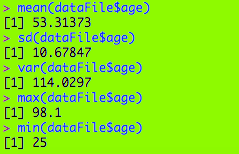
This is Michael, and today’s post will be on basic graphing with R. I’ll be using a different dataset for this post-murder_2015_final , which details the change in homicide rates from 2014 to 2015 as well as the individual homicide rates for 2014 and 2015 in 83 US cities (I felt this one was more quantitive than the dataset I used in my last two posts).

So let’s begin with a bar chart.

29Jun capture2

  • If you can’t read this, here’s the code
    • plot(file$X2015_murders, file$change, pch=20, col=”red”, main=”2014-2015 murder rate changes”, xlab=”2015 murders”, ylab=”Change from 2014 homicide rate”)

29Jun capture1

As you can see, there are two outliers at the upper-right hand corner of the screen. If you want to find out what those cities might be, here’s how you would add labels to each of the points.

1jul-capture2.png

  • Remember not to close the window with the graph when typing this command!

1Jul capture

From this graph, we can see that the two outliers (or cities with the largest 2014-to-2015 rise in murder rates) are Chicago and Baltimore.

Let’s try a bar graph now. Here’s the command to make a basic bar chart.

1Jul capture4

1Jul capture3

As you can see, 53 of the cities had a year-to-year rise in murder rates, 4 had no change in murder rates, and 26 had a year-to-year drop in murder rates (if you’re wondering what those cities are, check the spreadsheet attached to this post).

Let’s make another graph-the box plot. Here is the command

1Jul capture6

1Jul capture5

Some things to know when reading a box plot

  • The bold dashes represent the median value for the murders in a certain state (or only value if a state appears just once)
  • The top and bottom lines represent the lowest and highest values corresponding to a certain state
  • The yellow bars denote the range of the majority of values for a certain state
  • The dashed lines on the top and bottom of the chart show the highest and lowest values not in the range denoted by the yellow bar
    • If there aren’t any dashed lines, then the yellow bars denote all of the values, not just the majority
  • Any circles you see are outliers corresponding to a particular state.


One more thing, if you’re wondering where I got this data from, here the website-https://github.com/fivethirtyeight/data/blob/master/murder_2016/murder_2015_final.csv. The website is FiveThirtyEight.com, which writes interesting data-driven articles, such as  The Lebron James Decision-Making Machine. FiveThirtyEight then posts the code and data used in these articles on GitHub so anyone can perform statistical analyses on the data (good place to look for free datasets for your own data analysis project, and much more interesting than the free datasets that come with R with data 40+ years old).

Thank you,

Michael

R Lesson 2: Basic summarization of R Data

Hello everybody,

This is Michael, and today’s post will be about basic summarization of R Data. I thought this would be an appropriate place to continue from R Lesson 1: Basic R commands (I’ll be using the dataset from that post).

Let’s start off simple by using the summary() command to display a summary of the age field.

27Jun capture1

As you can see, the output shows the minimum age for any congressperson (25), the end of the 1st quartile (45.4), the median age (53), the mean age (53.31), the beginning of the third quartile (60.55), and the maximum age (98.1). But what does this all mean?

  • The minimum is obviously the minimum age amongst the congresspeople-25 years
  • The 1st quartile is the age between the minimum and the mean (45.4)
    • In other words, the youngest 25% of congresspeople were between 25 and 45.4 years old (at the start of their terms)
  • The median is the center of all the ages amongst the congresspeople-53 years in this case
    • 50% of congresspeople were between 45.4 and 60.55 years old (at the start of their terms)
  • The mean is the average of all the ages
  • The 3rd quartile is the age between the median and the maximum (60.55)
    • In other words, the oldest 25% of congresspeople were between 60.55 and 98.1 years old (at the start of their terms)
  • The maximum is obviously the maximum age amongst the congresspeople-98.1 years

However, if you use summary on a non-numeric field, such as state, the counts for each observation (in this case, how many times each state appears in the dataset).

27Jun capture2

Another summary command I will discuss is table(), which shows all values of a variable along with each values’ frequencies (how many times that value appears in the dataset).

Below is a table displaying the number of congresspeople who are representatives, as well as those who are senators.

27Jun capture3

Now here’s what the table would look like if we add another value (I’ll use congress)

27Jun capture4

Like the last table, this table shows the number of representatives and senators, except divided up by congress (80th to 113th specifically).

Thanks for reading,

Michael


R Lesson 1: Basic R commands

Hello everyone,

It’s Michael, and I thought a perfect first post (aside from my welcome post) would be an intro to the wonderful, statistical and completely free software known as R. The dataset I will use will be congress-terms.csv, which I have attached to this post.

To start we will first upload the file onto R. If you are wondering how to do that, here’s the command:

  • dataFile <- read.csv(“/Users/michaelorozco-fletcher/Downloads/congress-terms.csv”)

You may choose different a different variable name. Your file path will be different too. To know what your file path is, open up Excel, then click File > Properties. This window will pop up.

screengrab2

The location field would be your file path (along with a slash and the file name, congress-terms.csv in this case, after “Downloads”).

Allright, now that I explained how to read a CSV file onto R, here are some basic R commands.

screengrab1

str(dataFile) displays a summary of all the data fields in the file, which is important for understanding the data you are working with. As mentioned above, there are 18635 observations of 13 variables, which include

  • congress-which term of Congress does a particular congressperson serve in (anywhere from the 80th-lasting from 1947 to 1949-to the 113th-lasting from 2013 to 2015)
  • chamber-whether a particular congressperson is a part of the House or Senate
  • bioguide-each congressperson’s ID Number within the Biographical Directory of the United States Congress
  • firstname, middlename, lastname-These are self-explanatory
  • suffix-A “Jr.” or “III” or something like that at the end of a particular congressperson’s name
  • birthday-Again, self-explanatory
  • state-What state the congressperson serves
  • party-A congressperson’s party affiliation, whether D for Democrat, R for Republican, I for independent, among others
  • incumbent-whether a congressperson was in office at the beginning of a particular term (such as the 110th Congress) or came into office after another congressperson left
  • termstart-when a term of Congress began
  • age-how old a congressperson was when a term began


Now lets check out some other basic commands. I used the age field because it is the field with the most numbers.

screengrab3

Above you will find the mean, sd (standard deviation-square root of variance), var (variance-the standard deviation squared), max, and min for the age field. Some inferences we can make include

  • There is a fair spread among the ages (10.67 years, as given by sd)
  • The ages are quite spread out from the 53.31 mean (as given by the 114.03 var)
  • The oldest congressperson was almost 100 when his term began (J. Strom Thurmond, 1902-2003)

These are just a few of the basic commands. For more commands check out https://www.calvin.edu/~scofield/courses/m143/materials/RcmdsFromClass.pdf

Here’s the spreadsheet: congress-terms

Thank you,

Michael

Welcome

Hello readers,

My name is Michael, and this is my data science blog. Here you will find plenty of information about data science-ranging from how-to posts to analyses with actual datasets. I’ll mostly focus on MySQL, R, and Excel (with Java lessons from time to time) for now, though I may eventually add other analytical tools like Python.

Thank you,

Michael

interactive-line-graph