A Quick Lesson On CNNs, RNNs, and ANNs (AI pt. 4)

Hello everybody,

Michael here, and today, I thought I’d do something a little different. I won’t be doing any coding projects for today’s lesson, but since I’m currently doing an AI series of blog posts, I though I might take this post to explain the three main types of neural networks you’ll likely encounter in your AI work-CNNs, RNNs and ANNs.

All about ANNs

To begin our post on the three main types of neural networks, let’s first discuss ANNs, or artificial neural networks.

ANNs are the broadest type of neural network, as they encompass basically all types of neural networks. The aim of an ANN is to programaticially mimic the way the human brain thinks using plenty of tiny components that interact with each other-components which are otherwise referred to as artificial neurons (similar to the neurons in a human brain).

In simpler terms, the aim of ANNs is to teach the computer program to do things our brains can do, such as classify images, translate text from one language to another, and even detect people’s faces in an area.

A great example of an ANN can be seen below:

This is the homepage for my YouTube TV account, and above you’ll see a section called TOP PICKS FOR YOU. This is a reccommender section, as it uses an ANN to recommend programs that might be of interest to me based off of my viewing history (as of mid-January 2023). As you can see, the visible part of the TOP PICKS FOR YOU section has lots of cartoons and sports programming.

CNNs-A specific type of ANN

Next up, let’s explore CNNs, or convolutional neural networks, which are a type of ANN.

CNNs are neural networks that are often used for image analysis tasks such as identifying specific people/things in a picture and generating new images/videos from existing images/videos.

How exactly do CNNs work? Well, take a look at this brilliantly-rendered illustration I created on Microsoft Paint in about five minutes:

In this example, the CNN takes the image and utilizes several filtering layers, referred to as convolutional layers, to extract certain features from the image. As you can see from the above picture, this CNN is using four convolutional layers to extract four different features from the photo-face, location (the photo was taken), background (of the photo), and other things in the photo (like the color of my tie).

  • CNNs often utilize hundreds of convolutional layers-not just four-to extract features from an image.

The convolutional layers then take the details of each feature to generate new images containing these features. The generated images are then passed through multiple pooling layers, which bascially gather the gist of the information from the images generated from the convolutional layers. The CNN then uses fully connected layers to connect the information from both the convolutional layers and the pooling layers to classify objects in images.

Still not getting the gist of how CNNs work? Here’s an example that might help.

If you’ve got photos backed up to Google’s cloud, you’ve likely come across a feature that allows you to locate images based on the people or pets, places, or things that appear in the image. This feature is a great example of CNNs at work, as it uses CNNs to process an image, generate a new image from the original image, and use the information from the new generated image to identify the people, pets, places, or things in the image.

Aside from the Google Photos cloud example I just mentioned, another great example of a CNN can be seen in my previous two posts-Python Lesson 38: Building Your First Neural Network (AI pt. 2) and Python Lesson 39: One Simple Way To Improve Your Neural Network’s Accuracy (AI pt. 3). Since the MNIST classification neural network involved classifying images, in this case images of handwritten digits from 0-9, this neural network qualifies as a CNN.

RNNs-another type of ANN

Another type of ANN I wanted to discuss with you is RNNs, or recurrent neural networks. Unlike CNNs, which are mostly used for image analysis tasks, RNNs are used to analyze sequences of data such as text or audio.

How do RNNs work? Well, take a look at my other beautifully-rendered Microsoft Paint illustration to get a visual idea of how RNNs work:

In this example, we’re going to use Taylor Swift music to illustrate how RNNs work. To start the execution of the RNN, we’ll use music from four of Swift’s albums-Reputation, Midnights, Folklore, and Fearless-as input. In this RNN example, each of the albums would be initially processed through an input layer and further processed through a recurrent layer. Each recurrent layer creates connections that allow the information processed from the inputs to flow from one step of processing to the text. How do RNNs accomplish this seamless flow of information? The recurrent layers in RNNs store their “memory”, so to speak, of all the information that was processed from the inputs-the RNN’s “memory” works quite similarly to how our brain’s “memory” works. The RNN’s recurrent layers then use the data gathered from the information processing to generate an output-in this example, the output would be a new AI-generated Taylor Swift song (which, if you’re a Taylor Swift fan, might not enjoy).

Another great example of an RNN would be a chatbot, which is a program that utilizes an RNN to essentially have a conversation with you-a lot of businesses utilize them for customer service matters.

One famous chatbot you’ve likely come across recently is a little tool called ChatGPT, which looks like this:

For those unfamiliar, ChatGPT is a free AI chatbot launched by the AI research lab OpenAI on November 30, 2022. If you have used ChatGPT, you’ll be amazed at how smart and versatile it is. It can do things ranging from writing simple Python scripts (as seen in the screenshot above) to giving you dating advice and…well, the things ChatGPT can do warrants its own blog post (consider this a little preview of future content).

Combining CNNs and RNNs

Now, after reading my explinations of CNNs and RNNs, you might be wondering if you can build a tool combining both types of neural networks. The short answer here is yes-and I’ve got a well known example to prove it:

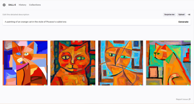
This is a neat, albeit controversial, tool called DALL-E. DALL-E utilizes both CNNs and RNNs to generate pictures based off of a text description. As you can see from the example above, DALL-E did quite a good job of generating a painting of an orange cat in the style of Pablo Picasso’s Cubist era. However, DALL-E’s accuracy in replicating Picasso’s style is also not without its ethical concerns, as it could threaten artists’ livelihoods due to its uncanny accuracy to replicate thousands of art styles.

As for the other things DALL-E can do…well, consider this another preview for a future blog post (because I think DALL-E’s capabilities also warrant its own blog post).

Thanks for reading,

Michael

Python Lesson 39: One Simple Way To Improve Your Neural Network’s Accuracy (AI pt. 3)

Hello everybody,

Michael here, and hope you all had a wonderful holiday season. I’ve got lots of exciting content planned for 2023-including something special for the blog’s 5th anniversary (yup, this blog turns 5 on June 13)-and I hope you all will follow along on this programming journey.

To start the year, I thought I’d pick up where I left off in 2022. If you recall, the last post I wrote in 2022 involved creating a basic neural network in Python using the famous MNIST dataset-Python Lesson 38: Building Your First Neural Network (AI pt. 2). In that post, you’ll also likely recall that the neural network we built had an accuracy of less than 20%. In this post, we’ll explore a simple way to improve that neural network’s accuracy. Let’s get coding!

A little refresher on our previous project

In case you’d like to see it again, here’s our code for the neural network project we made in the previous post:

import tensorflow as tf
import keras as kr
import tensorflow_datasets as tfds

(trainX, trainY), (testX, testY) = mnist.load_data()

trainX.shape
testX.shape
trainY.shape
testY.shape

import matplotlib.pyplot as plt
imageNum = 1500
plt.imshow(trainX[imageNum], cmap='magma')

import matplotlib.pyplot as plt
imageNum = 3332
plt.imshow(testX[imageNum], cmap='magma')

firstNeuralNetwork = tf.keras.models.Sequential([
    tf.keras.layers.Flatten(input_shape=(28,28)),
    tf.keras.layers.Dense(150, activation='relu'),
    tf.keras.layers.Dropout(0.2),
    tf.keras.layers.Dense(10)
])

firstNeuralNetwork.compile(optimizer='adam', loss='sparse_categorical_crossentropy', metrics=['accuracy'])
firstNeuralNetwork.fit(x=trainX,y=trainY, epochs=25)

firstNeuralNetwork.evaluate(testX, testY)

To recap, in this code, we built a basic neural network in Python to classify handwritten digits in the MNIST dataset and as I mentioned earlier, this model wasn’t very accurate. In fact, we didn’t acheive accuracy higher than 20% through any of the iterations. Let’s explore some ways we can change that.

One simple way to improve the neural network’s accuracy

Pay attention to this line of code-it creates the second Dense layer in our neural network (the layer that must have ten neurons in this example):

tf.keras.layers.Dense(10)

Similar to what we did for the first Dense layer, add an activation parameter when creating this dense layer (after the number 10). However, this time, set the value of the activation parameter to softmax, like so:

tf.keras.layers.Dense(10, activation='softmax')

You’re likely wondering, what is the softmax function? Here’s an easy way to explain it. Imagine you’re arranging a summertime trip and have four choices of departure dates-June 30, July 1, July 3, and July 5. Let’s say you wanted to use the softmax function to decide a departure date.

The way the softmax function works is that it takes the four aforementioned dates and assigns random probabilities to each of them-the sum of these four probabilites will equal 1 (essentially, we’re dividing the group of possible departure dates into four parts). In this example, let’s say the four probabilities assigned were 46% (for June 30), 20% (for July 1), 19% (for July 3), and 15% (for July 5). All of these probabilites add up to 1-or 100%.

Now that we’ve explained the softmax function, let’s see how it helps improve our neural networks accuracy without changing anything else in the code.

First, let’s see how the accuracy for each epoch is affected:

firstNeuralNetwork.compile(optimizer='adam', loss='sparse_categorical_crossentropy', metrics=['accuracy'])
firstNeuralNetwork.fit(x=trainX,y=trainY, epochs=25)

Epoch 1/25
1875/1875 [==============================] - 5s 2ms/step - loss: 2.4216 - accuracy: 0.7781
Epoch 2/25
1875/1875 [==============================] - 4s 2ms/step - loss: 0.5508 - accuracy: 0.8612
Epoch 3/25
1875/1875 [==============================] - 5s 3ms/step - loss: 0.4453 - accuracy: 0.8877
Epoch 4/25
1875/1875 [==============================] - 5s 3ms/step - loss: 0.3841 - accuracy: 0.9004
Epoch 5/25
1875/1875 [==============================] - 5s 2ms/step - loss: 0.3730 - accuracy: 0.9069
Epoch 6/25
1875/1875 [==============================] - 4s 2ms/step - loss: 0.3482 - accuracy: 0.9123
Epoch 7/25
1875/1875 [==============================] - 4s 2ms/step - loss: 0.3343 - accuracy: 0.9167
Epoch 8/25
1875/1875 [==============================] - 4s 2ms/step - loss: 0.3250 - accuracy: 0.9178
Epoch 9/25
1875/1875 [==============================] - 4s 2ms/step - loss: 0.3182 - accuracy: 0.9224
Epoch 10/25
1875/1875 [==============================] - 5s 2ms/step - loss: 0.3103 - accuracy: 0.9238
Epoch 11/25
1875/1875 [==============================] - 5s 2ms/step - loss: 0.3041 - accuracy: 0.9251
Epoch 12/25
1875/1875 [==============================] - 5s 2ms/step - loss: 0.3022 - accuracy: 0.9258
Epoch 13/25
1875/1875 [==============================] - 4s 2ms/step - loss: 0.2983 - accuracy: 0.9280
Epoch 14/25
1875/1875 [==============================] - 4s 2ms/step - loss: 0.2962 - accuracy: 0.9288
Epoch 15/25
1875/1875 [==============================] - 4s 2ms/step - loss: 0.2832 - accuracy: 0.9320
Epoch 16/25
1875/1875 [==============================] - 4s 2ms/step - loss: 0.2904 - accuracy: 0.9321
Epoch 17/25
1875/1875 [==============================] - 5s 3ms/step - loss: 0.2861 - accuracy: 0.9308
Epoch 18/25
1875/1875 [==============================] - 5s 3ms/step - loss: 0.2805 - accuracy: 0.9337
Epoch 19/25
1875/1875 [==============================] - 5s 2ms/step - loss: 0.2859 - accuracy: 0.9334
Epoch 20/25
1875/1875 [==============================] - 5s 3ms/step - loss: 0.2775 - accuracy: 0.9365
Epoch 21/25
1875/1875 [==============================] - 4s 2ms/step - loss: 0.2800 - accuracy: 0.9346
Epoch 22/25
1875/1875 [==============================] - 4s 2ms/step - loss: 0.2825 - accuracy: 0.9371
Epoch 23/25
1875/1875 [==============================] - 5s 3ms/step - loss: 0.2743 - accuracy: 0.9370
Epoch 24/25
1875/1875 [==============================] - 6s 3ms/step - loss: 0.2749 - accuracy: 0.9383
Epoch 25/25
1875/1875 [==============================] - 5s 3ms/step - loss: 0.2703 - accuracy: 0.9372

Well, that’s a significant improvement from the per-epoch accuracy from the previous post! I mean, 77.8% accuracy on just the first epoch is quite impressive-and by the 25th and last epoch-the model achieves 93.7% accuracy.

Now, let’s check out the overall accuracy of the model:

firstNeuralNetwork.evaluate(testX, testY)

313/313 [==============================] - 1s 2ms/step - loss: 0.4758 - accuracy: 0.9471

94.7% overall accruacy-all by adding a simple line of code! If you recall from the previous post, our model’s overall accuracy was just 10.5%.

Thanks for reading, and I can’t wait to share all of the exiciting programming content I have planned for you all in 2023!

Also, if there’s anything you can take away from this lesson, it’s that sometimes the smallest code changes can make a big difference in your program.