datascience18, Author at Michael's Programming Bytes

The Glorious Five-Year Plan Part One

Hello everybody,

Michael here, and today is a very big day for Michael’s Programming Bytes (or for the nostalgic and longtime readers, Michael’s Analytics Blog). Know why?

This little pet project of mine turns 5 today! Yes, five wonderful years ago, on June 13, 2018, I was just a month removed from college when I got the idea to start this very blog. Anyone remember my welcome post, aptly titled Welcome?

Reflections, reflections and a glimpse into my thought process these last five years…

Where do I begin? How did I start this blog?

OK, so I know I mention this blog’s origin story on my About page, but for those who don’t feel like navigating to the About page-or just want a quick summary of this blog’s story well, here it is.

As I mentioned earlier in this post, I launched this blog on June 13, 2018 with my Welcome message-my first official lesson was posted 12 days later on June 25, 2018. It was a very simple lesson on how to run basic R commands-here’s the link: R Lesson 1: Basic R commands.

Looking back on that first R lesson, I thought it was a very fitting way to begin my blogging journey. See, I’d been taking some really fun data analytics courses during my last semester of undergrad (this was Spring 2018, a few months before the launch). One such course was in R, which I was quite fascinated with (well, aside from the fact that there was a programming language called R).

After finishing undergrad in April 2018, I intially sought out data analytics jobs. However, I realized that I wanted to have an easy means to showcase my data analytics skills to potential employers. Hence, on June 13, 2018, I launched this blog-then known as Michael’s Analytics Blog.

If you’ve perused the entire 145-post catalog (and kudos if you have), you’ll likely have noticed that almost every single post from 2018-my first year active-is majority data analytics, though my long-lost MySQL series from fall 2018 does go into very very basic database building. There’s a good reason for that. Since I mentioned that I intially wanted a career purely in data analytics, I thought what better way to showcase my analytical skills than through writing? After all, I thought this could certainly double as my “data analyst portfolio”.

I know my earliest posts were purely analytical, but come the beginning of 2019, I wanted to explore other aspects of programming. With that said, on January 11, 2019, I wrote my first real non-analytical post-Java Lesson 1: Introduction to Java & “Hello World”. This post covered a very basic Java concept-System.out.println()-and the Hello world schtick most developers learn about when they first start learning about the craft of coding (if you’re a developer, odds are you’ll remember learning about how to print Hello world during your early coding days).

My first year of blogging only covered three major programming tools-Java, R and MySQL. After all, those were the only three programming tools I had any experience in coming out of college, so it’s not like I could cover more adavanced concepts. However, that changed once I began my tech job in the summer of 2019, as I also introduced Python into my blog’s repetoire with the post Python Lesson 1: Intro to Python on August 5, 2019.

As I gained more on-the-job and self-taught skills, I was able to cover more interesting programming topics (to me at least). Aside from Python, I was able to introduce HTML (February 2, 2021), GitHub (on the blog’s third anniversary), CSS (March 19, 2022), and Bootstrap (September 7, 2022). Throughout this blog’s five-year run, I’ve certainly broadened my focus from purely data analytics content to topics such as creating graphics, natural language processing, AI, web development, code management and much much more. To be honest, when I began this blog, I thought I’d still be posting purely analytics content five years in-after all, that was the intial aim of this blog and why the original name was Michael’s Anlaytics Blog.

However, I realized that as my programming knowledge grew, my blog’s content should expand in scope-and that’s exactly how things have played out. To be honest, I think it not only makes my blog more interesting to anyone who wants to read it (and binge the five years worth of posts) but also serves as a showcase for my versatile programming skills (and creativity too). In case you’ve read my entire blog catalog, I’ve covered 8 programming tools total (and that number will likely grow).

Throughout these last five years, I’ve made sure to keep my blog as interesting as possible for you all. As you might have noticed, I RARELY use the free datasets provided by tools such as R and Python. Why is that? It’s a personal creative choice on my part to ensure more interesting content for you all, my loyal readers. Let’s be honest, what would be a more interesting dataset to analyze-the one on petal and sepal width (if you know, you know) that’s been analyzed to death or one covering COVID in the early days of the pandemic (R Analysis 9: ANOVA, K-Means Clustering & COVID-19)? Throughout this blog’s run, I’ve included analyses on various topics such as COVID (in 2020), the 2020 NBA playoffs, the MCU, and much much more.

The one rare time I did use a pre-made dataset was for my Python MNIST 2-part post in 2022/2023 (Python Lesson 38: Building Your First Neural Network (AI pt. 2) and Python Lesson 39: One Simple Way To Improve Your Neural Network’s Accuracy (AI pt. 3)). However, I only did so because I felt that MNIST was a perfect way to get you all familiar with neural networks-plus, datasets for neural networks are considerably larger than datasets for other kinds of analyses, so I felt using a premade dataset was better in this situation. However, premade datasets will usually be the exception and not the rule for me, so for as long as I’m running this blog (which I hope will be for many years to come) I’ll try to keep things interesting for you all as much as I can.

Another thing I feel makes my blog stand out from the hundreds of other coding blogs out there is that most coding/tech blogs tend to specialize in one area of coding/tech, such as AI, Python, game development, etc. However, my blog is like a jack-of-all-coding trades-you don’t know what I’ll cover next. Plus, if you want to learn how to create amazing data visualizations, work with GitHub, analyze natural language through code, figure out how to solve calculus problems, work with basic web development, and so much more, this blog has you covered (and there’s certainly room to cover many, many more cool things in the long-term).

A 5-year message to you all

Unlike my 4th anniversary post, I don’t have any major updates for this blog (and no, another name change isn’t looming). However, before I go, I did want to leave you all with a message.

Oh, did I say I was gonna leave you with a message. Well, if you thought it was going to be some generic “thank-you-for-five-amazing-years” message, you’re wrong. Instead, to celebrate five years of Michael’s Programming Bytes/Michael’s Analytics Blog (however you want to refer to this blog), I’ve hidden my thank-you message in the form of a coding challenge. You ready?

Michael’s Five Year Coding Challenge

So, you think you’ve got what it takes to solve my five-year coding challenge and decode my five-year message? Before you begin problem solving, here’s the message I’d like you to decode:

Gszmp blf gl zoo nb ivzwvih uli urev dlmwviufo bvzih. R dlfowm'g szev pvkg gsrh yolt ifmmrmt uli zh olmt zh R wrw drgslfg blfi dlmwviufo hfkklig.

R slkv blf ovzimvw hlnvgsrmt zolmt gsv dzb gsvhv ozhg urev bvzih-zmw, svb, nzbyv blf tzrmvw z olev lu kiltiznnrmt (zmw kviszkh mvd qly hprooh) rm gsv kilxvhh. Gszg dlfow xvigzrmob nzpv nv z evib szkkb dirgvi. Sviv'h gl nzmb, nzmb nliv bvzih lu xlwrmt gltvgsvi!

Nrxszvo

But wait, here’s the best part…

…you, yes you, can help me solve this puzzle. Since it’s my five year blog anniversary, I thought I’d experiment with something new-a coding challenge where you (or any of my readers) can participate.

What might you get out of it? Well, I’ll pick my top five submissions to showcase on my next post (assuming I get at least five submissions, of course). Do you also run a coding/programming blog? Let me know and I’d be glad to give it a shoutout here.

Some things to keep in mind before I consider sharing your work

To celebrate five years of this blog, I thought I’d celebrate the larger spirit of coding (corny I know)! With that said, feel free to use any programming tool to solve this puzzle-even if I haven’t covered it here.
You have until June 21, 2023 at 12AM US Central Time to show me what you created. If you’re wondering what this cutoff means in your timezone, here’s a handy timezone converter-https://www.timeanddate.com/worldclock/converter.html.
Although I said you can solve this puzzle using any programming tool of your choosing, there are three rules I’d like you to adhere to:
- You MUST have the correct answer (which I will share in part 2, along with my approach for solving the problem).
- You MUST use a reverse substitution cipher to decode the message. If you don’t know what a reverse substitution cipher is, it goes something like this: A = Z, B = Y, C = X and so on until Z = A.
- You MUST send me both the code and the output (and please, please send the code in a .txt file)
- Send me your work to the email miketheblogger@outlook.com (yes, I have a separate email for blog matters). Also send me the outputs in whatever formats works best-be it on a .txt file, through screenshots, or really whatever works for you.

Also, before you send me your work, please fill out this questionairre-https://forms.office.com/Pages/ResponsePage.aspx?id=DQSIkWdsW0yxEjajBLZtrQAAAAAAAAAAAAZ__sEfXLlUNE5KRzZJWjNQQlYzTVFXR05TQVBXM0tNRy4u.

Thanks for reading, and be sure to keep an eye out for part 2 of my five-year anniversary celebration. Yes, I decided to pull an Avengers: Infinity War here (if you know, you know) and split my big five-year celebration post into two. After all, let’s keep the fun going for one more post! Can’t wait to see you solve the code (and don’t worry-I’ll share my answer in the next post)!

Michael

R Lesson 29: An Integral Part of R Calculus

Hello everybody,

Michael here, and in today’s post, I’ll be discussing an integral part of R calculus-integrals (see what I did there?).

The integral facts about integrals

What are integrals, exactly? Well, we did spend the last two posts discussing derivatives, which are metrics used to measure the rate at which one quantity changes with respect to another quantity (i.e. like the change in Rotten Tomatoes critic scores from one MCU movie to the next as we discussed in this post-R Lesson 27: Introductory R Calculus). Integrals, on the other hand, measure rates of accumulation of a certain quantity over time.

Simple enough, right? Well, is it possible to think of integrals as reverse derivatives? Yes it is! I did mention that derivatives measure change of a given quantity from point A to point B while integrals measure the accumulation of a quantity over a given time period (which could be from point A all the way to point XFD1048576). In the context of mathematical functions, derivatives break up a function into smaller pieces to measure the rate of change at each point while integrals put the pieces of the function back together to measure the rate of change across the entire duration of the function (which obviously can be infinity)

Calculating integrals, the manual way, part 1

Before we dive into R calculations of integrals, let’s first see how to calculate integrals, the manual way, by hand.

Let’s take this polynomial as an example:

Now, how would we calculate the integral of this polynomial. Take a look at the illustration below:

Just so you know, the polynomial in green is the integral of the original polynomial. With that said, how did we get the polynomial 3/4x^4-2/3x^3+2x^2-7x+C as the integral of the original polynomial?

First of all, just as we did with derivatives, we would need to calculate the integral of each term in the polynomial one-by-one. To do so, you’d need to add one to the exponent of each term, then divide that term by the new exponent. Still confused? Let me explain it another way:

The integral for 3x^3 would be 3/4x^4 since 3+1=4 and 3 divided by 4 is, well, 3/4.
The integral for -2x^2 would be -2/3x^3 since 2+1=3 and 2 divided by 3 is, well, 2/3.
The integral for 4x would be 2x^2 since 1+1=2 and 4 divided by 2 is 2.
The integral for -7 would be -7x since constants have a power of 0 and 0+1=1 (and anything divided by 1 equals itself)
You will likely have noticed an additional value in the integral that you may not be aware of-the constant C. I’ll explain more about that right now.

So, you may be wondering what’s up with the C at the end of the integral equation. Remember how earlier in this post I mentioned that you can think of derivatives as reverse integrals. You may recall that in our previous lesson-R Lesson 28: Another Way To Work With Derivatives in R-I discussed that during the process of calculating a derivative for a polynomial, the derivative of any constant in that polynomial is 0. This means that when finding the derivative of any polynomial, the constant disappears.

Now, since integrals can be considered as reverse derivatives, we should remember that when we integrate a polynomial, there was likely a constant that disappeared during differentiation (which I forgot to mention is the name of the process used to find the derivative of a polynomial). The C at the end of an integral represents the infinite number of possible constants that could be used for a given integral.

An integral illustration to this lesson

For my more visual learners, here is an illustration of how integrals work:

Just as a derivative would measure the change from one point to another in this curve, the integral would measure the area under the curve. The area in yellow represents the negative integral while the area in red represents the positive integral.

Still confused? Don’t worry-we’ll definitely go more in depth in this lesson!

Calculating integrals, the R way, part 2

OK, now that we’ve discussed how to calculate integrals the manual way, let’s explore how to calculate integrals the R way. You’ll notice that R won’t just spit out the integral of a given polynomial but rather calculate the integral using an upper and lower limit. Don’t worry-I’ll explain this more later, but for now, let’s see how the magic is done:

integral <- function(x) { 3*x^3-2*x^2+4*x-7 }
result <- integrate(integral, lower=1, upper=2)
result
5.583333 with absolute error < 6.6e-14

In this example, I’m showing you how R does definite integration. What is definite integration? Let me explain it like this.

In the previous section of this post, all we were trying to do was to calculate the integral polynomial of a certain expression. This is known as indefinite integration since we were simply trying to find the integration function of a given polynomial with the arbitrary constant C. As I mentioned in the previous section, the constant C could represent nearly anything, which means there are infinite possible integrals for any given polynomial.

However, with definite integration (like I did above), you’ll be calculating the integral at an upper and lower limit-this is certainly helpful if you’re looking for the integral over a specific range in the polynomial function rather than just a general integral, which can stretch for infinity. In R, to calculate the integral of a function over a given range, specify values for the lower and upper parameters (in this case I used 1 and 2). As you can see from the result I obtained, I got ~5.58 with an absolute error of 6.6e-14, which indicates a very, very, very small margin of error for the integral calculation. In other words, R does a great job with definite integration.

Keep in mind that the integration calculation approach I discussed above will only work with a finite range of integration (e.g. lower=1, upper=2). It won’t work with an infinite range of integration (e.g. from negative infinity to positive infinity).

Plotting an integration function

Now that we know how to calculate integrals, the next thing we’ll explore is plotting the integration function. Here’s how we’d do so-using the polynomial from the first section and an integration range of (0,5):

integral <- function(x) { 3*x^3-2*x^2+4*x-7 }
integrated <- function(x) { integrate(integral, lower=0, upper=50)$value }
vectorIntegral <- Vectorize(integrated)
x <- seq(0, 50, 1)
plot(x,vectorIntegral(x), xlim=c(0,50), xlab="X-values", ylab="Y-values", main="Definite Integration Example", col="blue", pch=16)

So, how did I manage to create this plot? Let me give you a step-by-step explanation:

I first set the function I wish to integrate as the value of the integral value.
I then retrieved the integral of this function at the range (0,5). I also grabbed the value of the integral at this range and nested this result into its own function, which I then stored as the value of the integrated variable.
I then vectorized the value of the integral at the range (0,5) and stored that value into the vectorIntegral variable.
I then created an x-axis sequence to use in my plot that contained the parameters (0, 50, 1) which represent the lower limit, upper limit, and x-axis increment for my plot, respectively. This sequence is stored in the x variable.
Last but not least, I used the plot() function to plot the integral of the polynomial 3x^3-2x^2+4x-7. One thing you may be wondering about is the x, vectorIntegral(x) parameter in the function. The x parameter gathers all the x values for the plot (in this case the integers 0 to 5) while the vectorIntegral(x) parameter calculates all of the correpsonding y-values for each possible x-value and gathers them into a vector, or array, for the plot.
- Why choose vectorization to calculate the corresponding y-values? Well, it’s easier than looping through each possible x-value in the integral range to get the correpsonding y-values, since vectorization simply takes in all possible x-values (0-50 in this case) as the input array and returns an output array containing all possible y-values for each possible x-value (which in this case all seem to be between 4,000,000 and 5,000,000).

Calculating integrals, the manual way, part 3

So, now that I’ve shown you how to do definite integration the R way, let me show you how to do so the manual way. Let’s examine this illustation:

So in this illustration, I’m trying to calculate the integral for the polynomial 3x^3-2x^2+4x-7 using the (7,10) range. How do I do so. Well, first I perform some indefinite integration by finding the integral of the given polynomial-only thing here is that I don’t need the constant C. Next, since my integration range is (7,10), I evaluate the integral function for x=10 and subtract that result from the result I get after evaluating the integral function for x=7. After all my calculations are complete, I get 5342.25 as the value of my integral (rounded to two decimal places) at the integration range of (7,10).

If you’re wondering what that weird-looking S means, that’s just a standard integral writing notation.
To calculate the integral of any given expression for a given range, always remember to first find the integral of the polynomial and then evaluate that integral for x=both the upper and lower limits. Subtract the result of the upper limit evaluation from the result of the lower limit evaluation. And remember that, as we saw in our R integral calculations, there will always be a very very very small margin of error.
In calculus function notation, the capital F represents the f(x) of the integral while the lowercase f represents the f(x) of that integral’s derivative.

Thanks for reading!

Michael

R Lesson 28: Another Way To Work With Derivatives in R

Hello everybody,

Michael here, and in today’s lesson, I’ll show you another cool way to work with derivatives in R.

In the previous post-R Lesson 27: Introductory R Calculus-I discussed how to work with derivatives in R. However, the derivatives method I discussed in that post doesn’t cover the built-in derivatives method R has to calculate derivatives…rather, methods R uses to calculate derivatives (there are two ways of approaching this). What might that method look like? Well, lets dive in!

Calculating derivatives, the built-in R way, part 1

Now, how can we calculate derivatives with the built-in R way? First, we’ll explore the deriv() function. Let’s take a look at this code below, which contains a simple equation for a parabolic curve:

curve <- expression(3*x^2+4*x+5)
print(deriv(curve, "x"))

expression({
    .value <- 3 * x^2 + 4 * x + 5
    .grad <- array(0, c(length(.value), 1L), list(NULL, c("x")))
    .grad[, "x"] <- 3 * (2 * x) + 4
    attr(.value, "gradient") <- .grad
    .value
})

In this example, I’m using the polynomial 3x^2+4x+5 to represent our hypothetical parabolic curve. To find the derivative function of this polynomial, I ran R’s built in deriv() function and passed in both the curve expression and "x" (yes, in double quotes) to find the derivative expression-as the derivative always relates to x (or whatever character you used to represent an unknown quantity). Now, as you see from the output given, things don’t look too understandable. However, pay attention to the second .grad line (in this case, 3 * (2 * x) + 4), as this will provide the derivative function of the parabolic curve equation-6x+4. We would use this equation to evaluate the rate of change between points in the parabolic curve.

Let’s say we wanted to evaluate the derivative polynomial-6x+4-at x=5. If we use this x value, then the derivative of the parabola at x=5 would be 34.

If you thought the output I’m referring to read as 3(2x)+4, you’d be wrong. Remember to multiply the 3 by the 2x to get the correct answer of 6x (6x+4 to be exact).
When you’re writing a polynomial in R, remember to include all the multiplication signs (*)-yea, I know it’s super annoying.

In case you wanted a visual representation of this parabola, here it is:

I created this illustation of a parabola using a free online tool called DESMOS, which allows you to quickly create a visual representation of a line, parabola, or other curve. Here’s the link to DESMOS-https://www.desmos.com/calculator/dz0kvw0qjg.

Calculating derivatives, the built-in R way, part 2

Now let’s explore R’s other built-in way to calculate derivatives-this time using the D() function. For this example, let’s use the same parabolic curve equation we used for the deriv() example:

curve <- expression(3*x^2+4*x+5)
print(D(curve, "x"))

3 * (2 * x) + 4

As you can see, we passed in the same parameters for the D() function that we used for the deriv() function and got a much simpler version of the output we got for the deriv() function-simpler as in the derivative expression itself was the only thing that was returned.

Since the derivative expression returned from the D() function is the same as the expression returned from the deriv() function,

Calculating derivatives, the manual way, part 3

Yes, I know I was mostly going to focus on the two built-in R functions used to calculate derivatives-deriv() and D()-but I thought I’d include this bonus section for those of you (especially those who enjoy exploring calculus) who were wondering how to manually calculate derivatives.

Let’s take the same polynomial we were working with for the previous two examples:

How would we arrive at the derivative expression of 6x+4? Check out this illustration below:

From this picture, here are some things to keep in mind when calculating derivatives of polynomials (and it’s not the same as calculating derivatives of regular numbers like we did in the previous post R Lesson 27: Introductory R Calculus):

Go term-by-term when calculating derivatives of polynomials. In this example, you’d calculate the derivative of 3x^2, then the derivative of 4x and lastly the derivative of 5.
How would you calculate the derivatives of each term? Here’s how (and it’s quite easy).
The derivative of 3x^2 would be 6x, as you would multiply the number (3) by the power (2) to get 6. You would then reduce power of the x^2 by 1 to get x (any variable in a polynomial without an exponent is raised to the power of 1). Thus, the derivative of 3x^2 would be 6x.
The derivative of 4x would simply be 4. Just as we did with 3x^2, we’d multiply the number (4) by the power (1) in this case to get 4. We would also reduce the power of x by 1 to simply get 4, since x has a power of 1 and 1-1=0. In a polynomial, constants (numbers without variables next to them) have a power of 0.
I mean, we could’ve written the derivative polynomial as 6x+4x^0, but 6x+4 looks a lot nicer.
As for the constant in this polynomial-5-it has a derivative of 0 since the derivative of a constant is always 0 (after all, any constant in a polynomial has a power of 0, so this makes perfect sense). Thus, the derivative of 5 isn’t included in the derivative polynomial of 6x+4.

Thanks for reading,

Michael

R Lesson 27: Introductory R Calculus

Hello everybody,

Michael here, and in today’s post, I’m going to revisit an old friend of ours-the language R. As you readers may recall, R was the first language I covered on this blog, and since we’re only a few posts away from the blog’s fifth anniversary, I thought it would be fun to revisit this blog’s roots as an analytics blog (remember the Michael’s Analytics Blog days everyone).

Today’s post will provide a basic introduction on doing calculus with R (including graphing). Why am I doing R calculus? Well, I wanted to do some more fun R posts leading up to the blog’s fifth anniversary and I did have fun writing the trigonometry portion of my previous post-Python Lesson 41: Word2Vec (NLP pt.7/AI pt.7)-that I wanted to dive into more mathematical programming topics. With that said, let’s get started with some R calculus!

Setting ourselves up

In this lesson, we’ll be using this dataset-

MCU-movies Download

This dataset contains the Rotten Tomatoes scores for all MCU (Marvel Cinematic Universe) movies from Iron Man (2008) to Guardians of the Galaxy Vol. 3 (2023). Both critic and audience Rotten Tomatoes scores are included for all MCU movies.

Now, let’s open up our R IDE and read in this CSV file:

MCU <- read.csv("C:/Users/mof39/OneDrive/Documents/MCU movies.csv", fileEncoding="UTF-8-BON")
> MCU
                                         Movie Year RT.score Audience.score
1                                     Iron Man 2008     0.94           0.91
2                              Incredible Hulk 2008     0.67           0.69
3                                   Iron Man 2 2010     0.71           0.71
4                                         Thor 2011     0.77           0.76
5           Captain America: The First Avenger 2011     0.80           0.75
6                                 The Avengers 2012     0.91           0.91
7                                   Iron Man 3 2013     0.79           0.78
8                          Thor The Dark World 2013     0.66           0.75
9          Captain America: The Winter Soldier 2014     0.90           0.92
10                     Guradians of the Galaxy 2014     0.92           0.92
11                     Avengers: Age of Ultron 2015     0.76           0.82
12                                     Ant-Man 2015     0.83           0.85
13                  Captain America: Civil War 2016     0.90           0.89
14                              Doctor Strange 2016     0.89           0.86
15               Guardians of the Galaxy Vol 2 2017     0.85           0.87
16                      Spider-Man: Homecoming 2017     0.92           0.87
17                              Thor: Ragnarok 2017     0.93           0.87
18                               Black Panther 2018     0.96           0.79
19                      Avengers: Infinity War 2018     0.85           0.92
20                        Ant-Man and the Wasp 2018     0.87           0.80
21                              Captain Marvel 2019     0.79           0.45
22                           Avengers: Endgame 2019     0.94           0.90
23                   Spider-Man: Far From Home 2019     0.90           0.95
24                                 Black Widow 2021     0.79           0.91
25   Shang-Chi and the Legend of the Ten Rings 2021     0.91           0.98
26                                    Eternals 2021     0.47           0.77
27                     Spider-Man: No Way Home 2021     0.93           0.98
28 Doctor Strange in the Multiverse of Madness 2022     0.74           0.85
29                      Thor: Love and Thunder 2022     0.63           0.77
30              Black Panther: Wakanda Forever 2022     0.84           0.94
31           Ant-Man and the Wasp: Quantumania 2023     0.47           0.83
32               Guardians of the Galaxy Vol 3 2023     0.81           0.95

As you can see, we have read the data-frame into R and displayed it on the IDE (there are only 31 rows here).

Now, before we dive into the calculus of everything, let’s explore our dataset:

Movie-the name of the movie
Year-the movie’s release year
RT.score-the movie’s Rotten Tomatoes score
Audience.score-the movie’s audience score on Rotten Tomatoes
R tip-when you are reading in a CSV file into R, it might help to add the fileEncoding="UTF-8-BON" parameter into the read.csv() function as this parameter will remove the junk text that appears in the name of the dataframe’s first column.

Calculus 101

Now, before we dive headfirst into the fun calculus stuff with R, let’s first discuss calculus and derivatives, which is the topic of this post.

What is calculus? Simply put, calculus is a branch of mathematics that deals with the study of change. Calculus is a great way to measure how things change over time, like MCU movies’ Rotten Tomatoes scores over the course of its 15-year, 32-movie run.

There are two main types of calculus-differential and integral calculus. Differential calculus focuses on finding the rate of change of, well, any given thing over a period of time. Integral calculus, on the other hand, focuses on the accumulation of any given thing over a certain period of time.

A good example of differential calculus would be modelling changes in a city’s population over a certain period of time; differential calculus would be used in this scenario to find the city’s population change rate over time. A good example of integral calculus would be modelling the spread of a disease over time (e.g. COVID-19) in a certain geographic region to analyze that region’s infection rate over a certain time period.

Now, what is a derivative? In calculus, the derivative is the metric used to measure the rate of change at any given point in the measured example. In this example, the derivative (or rather derivatives since we’ll be using two derivatives) would be the change in Rotten Tomatoes scores (both critic and audience) from one MCU movie to the next.

It’s R calculus time!

Now that I’ve explained the gist of calculus and derivatives to you all, it’s time to implement them into R! Here’s how to do so (and yes, we will be finding the derivatives of both critic and audience scores). First, let’s start with the critic scores derivatives:

criticScores <- MCU$RT.score
criticDerivatives <- diff(criticScores)
criticDerivatives

[1] -0.27  0.04  0.06  0.03  0.11 -0.12 -0.13  0.24  0.02 -0.16  0.07  0.07 -0.01 -0.04  0.07  0.01  0.03 -0.11  0.02 -0.08  0.15 -0.04 -0.11  0.12 -0.44  0.46 -0.19 -0.11  0.21 -0.37
[31]  0.34

To calculate the derivatives for each critic score, I first placed all of the critics’ scores (stored in the column MCU$RT.score) into the vector criticScores. I then used R’s built-in diff() function to calculate the difference in critic scores from one MCU movie to the next and-voila!-I have my 31 derivatives.

Even though there are 32 MCU movies, there are only 31 differences to calculate and thus only 31 derivatives that appear.

Calculating the derivatives of the audience scores works exactly the same way, except you’ll just need to pull your data from the MCU$Audience.score column:

audienceScores <- MCU$Audience.score
audienceDerivatives <- diff(audienceScores)
audienceDerivatives
 [1] -0.22  0.02  0.05 -0.01  0.16 -0.13 -0.03  0.17  0.00 -0.10  0.03  0.04 -0.03  0.01  0.00  0.00 -0.08  0.13 -0.12 -0.35  0.45  0.05 -0.04  0.07 -0.21  0.21 -0.13 -0.08  0.17 -0.11
[31]  0.12

Plotting our results

Now that we’ve calculuated the derivatives of both the critic and audience scores, let’s plot them!

Here’s how we’d plot the critic scores:

plot(1:(length(criticScores)-1),criticDerivatives, type = "l", xlab = "MCU Movie Number", ylab = "Change in critic score")

In this example, I used R’s plot() function (which doesn’t require installation of the ggplot2 package) to plot the derivatives of the critic scores. The y-axis represents the change in critic scores, while the x-axis represents the index for a specific MCU movie (e.g. 0 would be Incredible Hulk while 31 would be Guardians of the Galaxy Vol.3).

However, this visual doesn’t seem to helpful. Let’s see how we can fix it!

First, let’s create a vector of the MCU movies to use as labels for this plot:

movies <- MCU$Movie

Next, let’s remove Iron Man from this vector since it won’t have a derivative (after all, it’s the first MCU movie).

movies <- movies[! movies %in% c('Iron Man')]

Great! Now let’s revise our plot to first add a title:

plot(1:(length(criticScores)-1),criticDerivatives, type = "l", main="Changes in MCU movie critic reception", xlab = "MCU Movie Number", ylab = "Change in critic score")

You can see that the plot() function’s main paramater allows you to add a title to the graph.

Next let’s add some labels to our data points-remember to only run this command AFTER you have the initial graph open!

text(1:(length(criticScores)-1),criticDerivatives, labels=movies, pos=3, cex=0.6)

Voila! With the text() function, we’re able to add labels to our data points so that we can tell which movie corresponds with which data point!

Remember to include the same X and Y axes in the text() function as you did in the plot() function! In this case, the X axis would be 1:(length(criticScores)-1) and the Y axis would be criticDerivatives.

Now that we have a title and labelled data points in our graph, let’s gather some insights. From our graph, we can see that the critical reception for the MCU’s Phases 1 & 2 was up-and-down (these include movies from Iron Man to Ant-Man). The critical reception for MCU’s Phase 3 slate (from Captain America: Civil War to Spider-Man: Far From Home) was its most solid to date, as there are no major positive or negative derivatives in either direction. The most interesting area of the graph is Phases 4 & 5 (from Black Widow onwards), as this era of the MCU has seen some sharp jumps in critical reception from movie to movie. Some of the sharpest changes can be seen from Shang-Chi and the Legend of the Ten Rings to Eternals (a 44% drop in critic score) and from Eternals to Spider-Man: No Way Home (a 46% rise in critic score).

All in all, some insights we can gain from this graph is that MCU Phase 3 was its most critically well-recieved (and as some fans would say, the MCU’s prime) while the entries in Phase 4 & 5 have been hit-or-miss critically (ahem, Eternals).

Now that we’ve analyzed critic derivatives, let’s turn our attention to analyzing audience score derivatives. Here’s the plot we’ll use-and it’s pretty much the same code we used to create the updated critic score derivative plot (except replace the word critic with the word audience in each axis variable and in the title):

plot(1:(length(audienceScores)-1),audienceDerivatives, type = "l", main="Changes in MCU movie audience reception", xlab = "MCU Movie Number", ylab = "Change in audience score")

text(1:(length(audienceScores)-1),audienceDerivatives, labels=movies, pos=3, cex=0.6)

The change in audience reception throughout the MCU’s 15-year, 32-movie run looks a little different than the change in critic reception over that same time period. For one, there are fewer sharp changes in audience score from movie to movie. Also interesting is the greater number of positive derivatives in audience score for the MCU’s Phase 4 & 5 movies-after all, there were far more negative derivatives than positive for the MCU’s Phase 4 & 5 critical reception (this is also interesting because many fans on MCU social media accounts that I follow have griped about the MCU’s quality post-Avengers Endgame). One more interesting insight is that the sharpest changes in audience reception came during the peak of Phase 3 (namely from Black Panther to Avengers: Endgame). As you can see from the graph above, the change in audience reception is fairly high from Black Panther to Avengers: Infinity War then drops from Avengers: Infinity War to Ant-Man and the Wasp. The audience score drops even further from Ant-Man and the Wasp to Captain Marvel before sharply rising from Captain Marvel to Avengers: Endgame. I personally found this insight interesting as some of my favorite MCU movies come from Phase 3 (like Black Panther with its 96% on Rotten Tomatoes-critic score), though I do recall Captain Marvel wasn’t well liked when it came out in March 2019 (but boy oh boy was Avengers: Endgame one of the most hyped things of 2019).

Thanks for reading,

Michael

Python Lesson 41: Word2Vec (NLP pt.7/AI pt.7)

Hello everybody,

Michael here, and in today’s lesson, we’ll discover another AI NLP algorithm-word2vec (recall that a few posts back in Python Lesson 40: The NLP Bag-Of-Words (NLP pt. 6/AI pt.5) we discussed the bag-of-words algorithm).

What is the word2vec algorithm?

So, how does the word2vec algorithm work? Let’s say we were to process a text document using this algorithm. The word2vec algorithm would analyze each word in this document along with all other words commonly found near a certain word. For instance, if the word “family” was found in a document and the words “daughter”, “parents”, and “generations” were found near it-the word “family” would be lumped in with these words, as they are all related to each other.

If you were to ask your program for the three most similar words to “family” (according to our hypothetical document), it would say “daughter”, “parents” and “generations”. How would the word2vec algorithm find the most common words? By using a mathematical metric called cosine similarity-more on that later.

Preparing the data

So, before we dive into the magic of word2vec, let’s gather the data we’re going to use.

In this example, we’ll utilize this ChatGPT-generated essay below that contains five paragraphs on a very relevant topic in the year 2023-returning to the office-including both sides of the debate.

return-to-office-1 Download

So, let’s open up our Python IDEs and start coding!

First, let’s open and read this file into our IDE:

with open(r'C:\Users\mof39\OneDrive\Documents\return to office.txt', 'r', encoding='utf-8') as file:
    word2VecFile = file.read()
    print(word2VecFile)

In Favor of Returning to Office:

Many argue that returning to the office is crucial for maintaining the productivity and collaboration necessary for businesses to thrive. Working in the same space allows for easier communication, quicker decision-making, and better team building. It also provides opportunities for social interactions that can improve employee morale and job satisfaction.

Another benefit of returning to the office is the separation of work and home life. With many employees working remotely during the pandemic, the lines between work and personal time have become blurred. This can lead to burnout and other negative consequences. By returning to the office, employees can more easily maintain a work-life balance and avoid the mental exhaustion that comes with always being “on.”

Against Returning to Office:

On the other hand, many people argue that remote work has proven to be effective, and there is no need to return to the office. In fact, studies have shown that remote workers are often more productive than those who work in the office. Additionally, remote work allows for more flexibility in scheduling and reduces the amount of time and money spent commuting.

Another important consideration is the health and safety of employees. With the ongoing threat of COVID-19 and the emergence of new variants, returning to the office could put employees at risk. Some may not feel comfortable being in close proximity to their colleagues or may have concerns about the effectiveness of safety protocols. In these cases, continuing to work remotely may be the best option.

Ultimately, the decision to return to the office or continue remote work will depend on a variety of factors, including the type of work being done, the needs of the business, and the preferences of employees. It is important to consider all perspectives and prioritize the health and safety of everyone involved.

You can technically open a .txt file with the pd.read_csv method, but I prefer using the with...open method of reading .txt files since the pd.read_csv method outputs the text file in tabluar form, which isn’t going to work for this tutorial.

And now let’s create the word2vec model

Now that we’ve read our text file into the system, the next thing we’ll do is create our word2vec model. Here’s the code to do so:

First, lets gather our list of tokens for the analysis:

import nltk
import gensim

modelData = []
punctuation = [',', '.', '”', '“', ':']

for w in nltk.sent_tokenize(word2VecFile):
    tokens = []
    
    for t in nltk.word_tokenize(w):
        if t not in punctuation:
            tokens.append(t.lower())
        
    modelData.append(tokens)
    
print(modelData)

[['in', 'favor', 'of', 'returning', 'to', 'office', 'many', 'argue', 'that', 'returning', 'to', 'the', 'office', 'is', 'crucial', 'for', 'maintaining', 'the', 'productivity', 'and', 'collaboration', 'necessary', 'for', 'businesses', 'to', 'thrive'], ['working', 'in', 'the', 'same', 'space', 'allows', 'for', 'easier', 'communication', 'quicker', 'decision-making', 'and', 'better', 'team', 'building'], ['it', 'also', 'provides', 'opportunities', 'for', 'social', 'interactions', 'that', 'can', 'improve', 'employee', 'morale', 'and', 'job', 'satisfaction'], ['another', 'benefit', 'of', 'returning', 'to', 'the', 'office', 'is', 'the', 'separation', 'of', 'work', 'and', 'home', 'life'], ['with', 'many', 'employees', 'working', 'remotely', 'during', 'the', 'pandemic', 'the', 'lines', 'between', 'work', 'and', 'personal', 'time', 'have', 'become', 'blurred'], ['this', 'can', 'lead', 'to', 'burnout', 'and', 'other', 'negative', 'consequences'], ['by', 'returning', 'to', 'the', 'office', 'employees', 'can', 'more', 'easily', 'maintain', 'a', 'work-life', 'balance', 'and', 'avoid', 'the', 'mental', 'exhaustion', 'that', 'comes', 'with', 'always', 'being', 'on.', 'against', 'returning', 'to', 'office', 'on', 'the', 'other', 'hand', 'many', 'people', 'argue', 'that', 'remote', 'work', 'has', 'proven', 'to', 'be', 'effective', 'and', 'there', 'is', 'no', 'need', 'to', 'return', 'to', 'the', 'office'], ['in', 'fact', 'studies', 'have', 'shown', 'that', 'remote', 'workers', 'are', 'often', 'more', 'productive', 'than', 'those', 'who', 'work', 'in', 'the', 'office'], ['additionally', 'remote', 'work', 'allows', 'for', 'more', 'flexibility', 'in', 'scheduling', 'and', 'reduces', 'the', 'amount', 'of', 'time', 'and', 'money', 'spent', 'commuting'], ['another', 'important', 'consideration', 'is', 'the', 'health', 'and', 'safety', 'of', 'employees'], ['with', 'the', 'ongoing', 'threat', 'of', 'covid-19', 'and', 'the', 'emergence', 'of', 'new', 'variants', 'returning', 'to', 'the', 'office', 'could', 'put', 'employees', 'at', 'risk'], ['some', 'may', 'not', 'feel', 'comfortable', 'being', 'in', 'close', 'proximity', 'to', 'their', 'colleagues', 'or', 'may', 'have', 'concerns', 'about', 'the', 'effectiveness', 'of', 'safety', 'protocols'], ['in', 'these', 'cases', 'continuing', 'to', 'work', 'remotely', 'may', 'be', 'the', 'best', 'option'], ['ultimately', 'the', 'decision', 'to', 'return', 'to', 'the', 'office', 'or', 'continue', 'remote', 'work', 'will', 'depend', 'on', 'a', 'variety', 'of', 'factors', 'including', 'the', 'type', 'of', 'work', 'being', 'done', 'the', 'needs', 'of', 'the', 'business', 'and', 'the', 'preferences', 'of', 'employees'], ['it', 'is', 'important', 'to', 'consider', 'all', 'perspectives', 'and', 'prioritize', 'the', 'health', 'and', 'safety', 'of', 'everyone', 'involved']]

Before creating our tokens lists to use for our model, I first imported the nltk and gensim packages (as always, if there’s a required package you don’t have, pip install it!).

I then created two lists, modelData and tokens. Then I sentence-tokenized this file before word-tokenizing it, appending MOST of the tokens to the tokens list before appending each tokens list to the modelData list. I say appending MOST (not all) of the tokens as I excluded any tokens that were part of the punctuation list.

Now, you may be wondering if we should remove stopwords here like we’ve done for our previous NLP tutorials. Normally, I’d say yes, but since the text is so short and we’re trying to figure out word connections, I’d say keep the stopwords here to get more accurate word2vec results.

Now that we’ve got our tokens list-or should I say lists-within-a-list-it’s time to build our model!

Rather, I should say model(s), since there are two approaches we can take to build our word2vec analysis-skipgrams and continous-bag-of-words.

Skip-gram

The first word2vec approach we’ll explore is the skip-gram model.

What exactly is the skip-gram model, though? Using our text file as an example, let’s say we were trying to guess which words we’d commonly see before and after the word “working”. The skip-gram model would analyze our text file to guess which words we’d likely see before and after the word “working” such as “remotely” or “hardly”.

Now, how do we implement this model in Python? Take a look at the code below:

skipGram = gensim.models.Word2Vec(modelData, min_count = 1, vector_size = 2, window = 5, sg = 1)

What do each of these parameters mean. Let me explain:

min_count-sets the minimum amount of times a word must appear in a document to be factored into the skip-gram analysis; in this example, a word must appear in the document at least once to be factored into the skip-gram analysis
vector_size-sets the number of dimensions that each word vector will contain; in this example, each word vector will contain 2 dimensions
window-sets the maximum distance between current and predicted words in the document; this skip-gram analysis will look at the five words following and preceding any given word to determine cosine similarity (more on that later)
sg-if this value is 1, use the skip-gram analysis; if this value is 0, use the continous bag-of-words analysis (more on that later)

Now that we have our skip-gram word2vec model set up, let’s test it on three word pairs:

print("Cosine similarity between 'returning' and 'office' - Skip Gram : ", skipGram.wv.similarity('returning', 'office'))     
print("Cosine similarity between 'remote' and 'covid-19' - Skip Gram : ", skipGram.wv.similarity('remote', 'covid-19'))
print("Cosine similarity between 'reduces' and 'commuting' - Skip Gram : ", skipGram.wv.similarity('reduces', 'commuting'))

Cosine similarity between 'returning' and 'office' - Skip Gram :  0.9542125
Cosine similarity between 'remote' and 'covid-19' - Skip Gram :  -0.8962952
Cosine similarity between 'reduces' and 'commuting' - Skip Gram :  0.9316714

In this example, we are analyzing the cosine similiarty between three word pairs-returning & office, remote & covid-19 and reduces & commuting. As you can see from the output, two of the word pairs have positive cosine similarity while the other word pair has negative cosine similarity.

What does positive and negative cosine similarity mean? Well, the higher the positive cosine similarity, the more semantically similar the two words are to each other (in the context of the document being analyzed). The lower the negative cosine similarity, the more dissimilar the two words are to each other (again, in the context of the document being analyzed).

Just a tip, but using a vector_size of 2 is often not ideal, especially because most NLP analyses work with larger documents. I used a vector_size of 2 here because the document we’re working with is rather small.
Using a vector size of 0 or 1 won’t work for either the skip-gram or continuous bag-of-words model, as it will return cosine similarities of 1, -1, or 0, which aren’t ideal for your analysis.

Continuous bag-of-words

Now that we’ve explored the skip-gram model, let’s now analyze the continous bag-of-words model.

What is the continuous bag-of-words model? Well, like the skip-gram model, the continuous bag-of-words model is like a word2vec guessing game. However, while the skip-gram model attempts to predict words that will come before and after a given word, the continuous bag-of-words model will analyze a sentence in a document and try to predict what any given word in a sentence would be based on the surrounding words in the sentence.

Here’s a simple example:

The happy couple decided to close on their first _____ yesterday, eagerly anticipating all the memories they would make there.

Just from this sentence alone, what do you think the missing word would be? If you guessed house, you’d be right! In this example, the continuous bag-of-words model would look at each word in the sentence and based on the given words, guess the missing word.

Now let’s see how to implement the CBOW (continuous bag-of-words) model in Python.

CBOW = gensim.models.Word2Vec(modelData, min_count = 1, vector_size = 2, window = 5, sg = 0)

Now, here’s the best part about the CBOW model-it’s same up in exactly the same way, with the same parameters, as the skip-gram model. The only difference between the two models is that you’d need to set the sg parameter to 0 to indicate that you’d like to use the CBOW model.

Now let’s test our CBOW word2vec model on the same three word pairs we used for the skip-gram model.

print("Cosine similarity between 'returning' and 'office' - Skip Gram : ", CBOW.wv.similarity('returning', 'office'))     
print("Cosine similarity between 'remote' and 'covid-19' - Skip Gram : ", CBOW.wv.similarity('remote', 'covid-19'))
print("Cosine similarity between 'reduces' and 'commuting' - Skip Gram : ", CBOW.wv.similarity('reduces', 'commuting'))

Cosine similarity between 'returning' and 'office' - Skip Gram :  0.95738184
Cosine similarity between 'remote' and 'covid-19' - Skip Gram :  -0.9320767
Cosine similarity between 'reduces' and 'commuting' - Skip Gram :  0.94031644

Assuming a change in word2vec model but leaving all other parameters unchanged, we can see that the cosine similarity scores between the three word pairs show small differences from the skip-gram cosine similarity scores for the same three word pairs.

Cosine similarity explained

So, now that I’ve shown you all what cosine similarity looks like, it’s time to explain it further.

In the word2vec algorithm (for both the skip-gram and CBOW models), each word in the document is treated like a vector. Still unsure about the whole vector thing? Here’s an illustration that might help:

Imagine a simple right triangle, where the three words returning, office, and working are the angles. A and B are the sides while C is the triangle’s hypotenuse.

Let’s say you wanted to find the cosine similarity between the words returning and office. If you know even basic trigonometry, you’ll know that the cosine of a right triangle is the ratio of the length of the side adjacent to a given angle to the length of the triangle’s hypotenuse. The cosine would represent the cosine similarity between these two words.

In word2vec, cosine similarity scores can range from -1 to 1. Here’s an illustration on cosine similarity scores:

In simple terms, a word pair with a cosine similarity score of -1 or 0 indicates completely different, not-at-all semantic similar words (in the context of the document being analyzed). A word pair with a cosine similarity score greater than -1 but less than 0 indicates that the two words are somewhat, but not entirely, dissimilar. Finally, a word pair with a cosine similarity score of 1 indicates that the two words are identical or very, very similar semantically.

In the example above, the words returning and office have cosine similarity scores of roughly 0.95 (for both the skip-gram and CBOW models), indicating that these two words are quite semantically similar in the context of the document. Interestingly, the words remote and covid-19 have cosine similarity scores lower than -0.85 (for both the skip-gram and CBOW models)-personally I find this interesting as the word remote seems semantically similar to the word covid-19 in the context of this document (to me at least).

How is negative cosine similarity possible? Well, think of an obtuse traingle. In an obtuse triangle, one angle has to be greater than 90 degrees, which means the cosine of that angle can possibly be negative. Think of NLP cosine similarity the same way.

Thanks for reading,

Michael

Michael’s New Spinoff Blog!

Hello readers,

It’s Michael, and I’ve got a super cool blog announcement for you all! I know you all wanted some more neural network/AI content, but please here me out here!

So as most of you know, I launched this blog on June 13, 2018, which means that I’ve been keeping up this blog for almost five years now. Through the course of writing 140 blog posts, I thought it would be time to expand the Michael’s Programming Bytes brand.

You may be wondering, how do I plan to expand my brand? Well, I figured that today, April 1, 2023, would be the perfect day to announce my very-first spinoff blog-Michael’s Poetic Programming Bytes! Yes, I thought I’d combine all the fun of coding with the simple creative joy of poetry.

What can you, the readers, expect from my first foray into creative writing? Well, we’ve got odes to the joy of coding:

Oh, joy of programming, how sweet your song,
With every keystroke, we dance along.
A world of code at our fingertips,
Endless possibilities, endless trips.

With loops and functions, we craft our art,
A symphony of logic, a work of heart.
Each line a brushstroke, each file a canvas,
We paint our dreams with logic and balance.

The bugs may bite, the code may crash,
But we rise above and make a dash.
To debug and fix, to learn and grow,
And create a masterpiece, a thing of flow.

Oh, joy of programming, you bring us delight,
A world of creation, a world of might.
We tinker and play, we solve and code,
And with each project, we find our abode.

So let us embrace this world of code,
And let our imaginations be bestowed.
With the joy of programming, we can create,
A world of wonder, a world of fate.

Haikus for those who enjoy this form of poetry, like this one about COBOL:

Legacy language,
COBOL endures through the years,
Business still needs it.

Looking for a fun way to learn about basic coding concepts? Michael’s Poetic Programming Bytes has content for that, like this Shakespearan sonnet explaining the concept of object-oriented programming:

Oh, wondrous world of code, how strange thy ways,
Wherein doth dwell the art of programming,
And rules of logic shape the programmer's days,
While algorithms bring life to every thing.

And yet, there lies a path less traveled by,
A new approach to programming art sublime,
Where objects are the stars that light the sky,
And classes, their domains, rule space and time.

Behold, the paradigm that we call OOP,
Where objects are defined by their attributes,
And methods grant them power, this we do see,
As they perform actions and execute.

Thus, OOP is a world of boundless creation,
Where objects reign supreme, in this new nation.

Or, if you want something a little more modern, here’s a rap about about why you shouldn’t use star imports in Python:

(Intro)
Listen up, y'all, it's time to learn
'Bout Python code and what to discern
We talkin' star imports, don't you know
Why you shouldn't use 'em, I'll tell you so

(Verse 1)
Star imports may seem like a good choice
But let me tell you, it's not worth the noise
You import everything, all at once
But that's a recipe for a coding dunce

'Cause when you import, you want to be clear
What you need, and what you don't want near
But with star imports, it's all or none
And that's not the way to get it done

(Hook)
So don't use star imports, take your time
Import what you need, it's not a crime
Cleaner code, that's what you'll get
And that's the key, you can bet

(Verse 2)
Now let's talk about naming collisions
With star imports, you risk some divisions
Two modules with the same name
Now you got a problem, that's not a game

You gotta qualify the name, make it clear
Which module you want, or it won't adhere
And if you got a lot of imports, it's a mess
So don't use star imports, that's my address

(Hook)
So don't use star imports, take your time
Import what you need, it's not a crime
Cleaner code, that's what you'll get
And that's the key, you can bet

(Bridge)
Now you know the deal, you gotta be wise
Don't take shortcuts, that's not the prize
Clean code is what we strive for
So don't use star imports, that's the score

(Hook)
So don't use star imports, take your time
Import what you need, it's not a crime
Cleaner code, that's what you'll get
And that's the key, you can bet

(Outro)
Yeah, that's right, don't use star imports
Import what you need, that's the report
Clean code, that's the goal
And with Python, you're in control!

I don’t know about you, but I think that’s a good hook!

Feeling a little nostalgic for your favorite old software? We’ve got poems for that too, like this one mourning the loss and remembering the life of Python 2 (which was retired in 2020):

Oh Python 2, we bid thee farewell
With heavy hearts and a mournful knell
For all the years we spent with thee
Were filled with joy and camaraderie

But now the time has come to part
And let Python 2 depart
For though we loved thee to the end
It's time for Python 3 to ascend

Oh how we'll miss thy simple ways
Thy elegance and thy concise phrase
But now we must embrace the new
And bid thee fond adieu

So let us honor thee this day
And remember all the fun we had along the way
We'll miss thee dearly, that much is true
But in our hearts, we'll always remember Python 2.

Michael’s Poetic Programmic Bytes will not only allow you to mourn the losses of your favorite programming tools, but also any piece of software that was near and dear to your heart, like this farewell tribute to Club Penguin (of which I never got into):

Dear Club Penguin, the time has come
To say goodbye, our hearts are numb
We'll miss the island and the snow
And all the friends we've come to know

For years we've waddled on your shores
Played mini-games and explored
Dressed up in our penguin clothes
And danced in clubs with puffle bows

You gave us endless hours of fun
And taught us lessons, one by one
To always be kind and to share
And help others, to show we care

We'll miss your parties and your quests
And all the joy that you expressed
But as we say our last goodbye
We'll keep your memory alive

So thank you Club Penguin, for it all
For the laughter and the thrill
We'll never forget the love we felt
For you, and always will.

Last but certainly not least, this blog will allow you to submit your own programming-themed poems that I’d love to showcase, such as this one on the joys of HTML written by a first-grader:

HTML, oh HTML,
You make websites so pretty,
With colors and pictures and text,
You make the internet look so witty!

I love how you make things bold,
And add links to click and see,
It's so cool to make a webpage,
With you, it's easy as can be!

Sometimes I forget a tag,
And my page looks kinda funny,
But I know I can always fix it,
And make my site look sunny!

HTML, oh HTML,
You're my favorite thing to code,
I'll keep making webpages with you,
And sharing them all over the globe!

Or this gem from a 60-year-old celebrating the life of dial-up Internet:

Dial-up, oh dial-up,
You were slow but steady,
You brought the world to our fingertips,
And made us feel so heady.

With your hissing and buzzing sounds,
And the beeps that signaled our connection,
We knew we were in for a wait,
But we savored every moment of your affection.

You were our gateway to the internet,
A time when things were simpler,
We couldn't stream or download much,
But you gave us the world on a platter.

I remember waiting for pages to load,
And watching as images took shape,
It was a different time, a slower time,
But one that we embraced.

Now we have fiber and Wi-Fi,
And we can stream without a hitch,
But I'll always remember dial-up,
And the way you made us rich.

Dial-up, oh dial-up,
You may be a relic of the past,
But your memory lives on in our hearts,
A time that will always last.

Wow-that’s a beautifully written tribute to the joys of dial-up internet (hey, I’m just 27 and still recall the dial-up days).

So if you’re ever in the mood to learn basic coding concepts or just pay homage to your favorite programming tools or software (ahem Club Penguin fans), then you’ll definitely enjoy Michael’s Poetic Programming Bytes with a whole library of poems that were certainly not spit out of an AI chatbot.

More details on this expansion of the Michael’s Programming Bytes brand to come, and also,

Will this be a new Michael’s Programming Bytes tradition? Time will tell.

And Now Let’s Create Some AI Art! (AI pt.6)

Hello everybody,

Michael here, and today’s post will be a little different than my previous posts. First of all, I know you all are looking forward to more neural network content-and don’t worry, I’ll deliver on that! However, while I get that content ready, I thought I’d do something a little fun for you all by experimenting the popular AI art tool DALL-E 2.

An intro to DALLE 2

We’ll start our journey down the AI art rabbit hole by first discussing the basics of DALLE 2.

First of all, what is DALLE 2? Well, DALLE 2 is the second version of the DALLE AI art algorithm-both DALLE and DALLE 2 were created by OpenAI-the same lab that created the ChatGPT chatbot. In fact, ChatGPT and both iterations of the DALLE art algorithm utilize the GPT (or Generative Pre-Transformer) NLP neural network. The original iteration of DALLE was released in January 2021 and DALLE 2 was released as a beta test in July 2022.

Setting up DALLE 2

Now, how would you start using DALLE 2? First of all, click on this link to be navigated to DALLE’s homepage-https://openai.com/product/dall-e-2:

Once you get to the DALLE 2 homepage, click on the Try DALLE link to start working with DALLE 2. Once you click on this link, you’ll need to sign up for a free DALLE 2 account (if you have a Gmail account, you can simply use these credentials for signing up).

After signing up for a DALLE 2 account, you’ll see a screen that looks like this:

Once you see this screen, you can type a prompt into the text box and have fun creating AI art!

If you haven’t figured out where the name DALLE 2 comes from, it’s simply a portmanteau of the artist Salvador Dali and the PIXAR robot WALL-E (which was a great movie by the way).
You only get 15 free DALLE 2 prompts a month, so use them wisely. Of course, you can always pay for more prompts if you feel inclined to do so-the cheapest deal is 115 prompts for $15 (not bad).

And now let’s create some AI art!

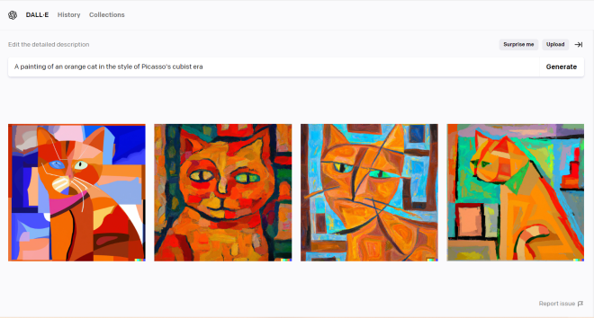
Let’s start with a simple DALLE 2 prompt-perhaps A coloring book page featuring two tabby cats and a ball of yarn. Here’s the output we get:

As you can see, DALLE 2 does quite a great job of creating a coloring book page featuring two tabby cats and a ball of yarn-it even returns one partially colored page.

This prompt, along with any other prompt you type into the input box, will generate four AI art images based off of what you typed into the input box.

Now, let’s try this prompt-A painting of a cow jumping over the moon in the style of Andy Warhol-and see what kind of output we get:

As you can see, DALLE 2 did quite a good job of creating an Andy Warhol-style painting of a cow jumping over the moon. If you’re familiar with Warhol’s work, you’ll be amazed at how well the DALLE 2 algorithm replicates his style (though I would be remiss not to note that DALLE 2’s amazing ability to recreate any art style isn’t without controversy, as this algorithm can easily mimic many art styles without the consent of the artists).

AI art still has a long ways to go

Look, DALLE 2 is smart enough (or rather, built well enough) to generate thousands and thousands of images by working its deep learning magic to mimic thousands of different art styles. But-at least as of March 2023-AI art is still far from perfect.

Let’s say we wanted to generate an AI image of an ice cream shop with the sign Mike's Ice Cream Shop with DALLE 2. Here’s what happens:

In this example, I used the prompt A colored pencil sketch of an ice cream store with a sign that says "Mike's Ice Cream Shop". The four art pieces that were generated create great colored-pencil sketches of an ice cream shops, but none of the storefront signs say “Mike’s Ice Cream Shop”, which is part of the request I sent to DALLE 2. Rather, all the signs generated contain gibberish text (my favorite one is the second picture which has a sign reading “Mik Mic Shke”).

OK, so DALLE 2 can’t really generate a good sign for my made-up ice cream store, but can it generate a good logo for this blog? Let’s find out:

OK, so I asked DALLE 2 to generate a logo for this blog and include the blog’s name-Michael’s Programming Bytes-and its slogan-“Byte sized programming classes for all coding learners”-on the logo. Much like the “Mike’s Ice Cream Shop” example above, the four logos generated don’t contain either the blog’s name or slogan. What the AI-genreated logos contain, however, is a lot of gibberish (though if I ever created a blog called “Mtheglyles” with the slogan “Byilyse”, I’d certainly use the first AI-generated logo).

So, we can see that DALLE 2 isn’t so good with inserting string of text into its AI-generated art. However, can DALLE 2 generate images of people? Let’s find out:

In this example, I typed in the prompt A watercolor painting of President Joe Biden and as you can see from the lack of output above, my request was denied by DALLE 2.

If you click the content policy hyperlink, you’ll be redirected to DALLE 2’s content creation policy, which would give you a better idea as to why this request was denied:

As you can see from the content policy screenshot above, this request was denied because DALLE 2 generally doesn’t accept politically-themed prompts and my Joe Biden prompt fell into that category.

Now, let’s try another prompt that contains a public figure, but this time, let’s make it a non-political public figure. Take a look at the prompt below:

In this example, I used the prompt A photo of a movie poster with Ryan Reynolds' face on it and DALLE 2 generated four images of movie posters with what it thinks is Ryan Reynolds’ face on it. Granted, just like with the ice cream store example, the text on these AI-generated movie posters is pure gibberish, but the face on the first AI-generated poster does resemble Ryan Reynolds pretty closely. The face on the second poster bears somewhat of a resemblance to Reynolds while the third face (and especially the fourth face) looks almost nothing like him.

Interestingly enough, when I swapped Ryan Reynolds’ name (but left the rest of the prompt unchanged) for a female actress-Gal Gadot-this is what I got:

My best guess as to why DALLE 2 will generate images of some public figures (without 100% accuracy) and not others is, aside from their content policy, that OpenAI (the lab that makes DALLE 2) doesn’t want it to be too easy for people to make deepfakes-which in this day and age, would be a fair reason to make it hard to generate fully-accurate images of public figures.

Now that we’ve discovered the limits of DALLE 2 when it comes to generating images of public figures, let’s see how this algorithm does when it comes to generating images of general people:

In this example, I used the prompt A photo of friends on a college campus and the AI-generated results have been quite hit-or-miss. Granted, DALLE 2 did a good job of generating the background-a generic college campus in this case-but DALLE 2 didn’t quite have the same magic when it came to generating images of the people. Let’s take a closer look at one of those images (to take a closer look at an image, simply click on it):

As you can see in this image above, DALLE 2 did a great job of generating the background-a generic college campus-but didn’t do such a good job of generating the generic college students (especially the students’ faces). Also, if you zoom into this picture really closely, you’ll see that the young lady in the orange tank-top has six fingers on one hand.

Yes, even AI has its biases

Aside from DALLE 2’s sometimes imperfect art generations, another thing to note about this algorithm (and AI at large) is that, just like humans, AI has its biases too.

Are you familiar with unconscious bias? If not, it’s a phenomenon that affects how you behave around other people based off of assumptions and/or beliefs you may have about other people just based off of appearances (e.g. baggy clothes, skin color, etc.) rather than their character.

Well, AI does have its unconscious biases too. Think about it-who do you need to create and maintain AI infrastructure? Humans! Since humans have their unconscious biases, they can often incorporate their biases into the programs that they create (though I’m sure this isn’t true for every programmer/developer).

Let’s observe AI bias in action through this DALLE 2 prompt:

So the prompt I used-An oil painting of an American rapper-seems quirky enough, right? Well, take a look at the four AI-generated images and tell me what they have in common. Since all the AI-generated paintings are of black men, this does look like a clear example of unconscious bias in AI.

Let’s try one more example:

OK, so I used the prompt A photo of a kindergarten teacher and surprisingly, got less biased photos than I did in the previous example (but still, 3/4 of the AI-generated photos are of women, and not a ton of diversity in the AI-generated photos).

Interestingly enough, AI seems to fine generating images of people when it’s a single person. When there are multiple people in the picture (as you saw with our college friends example), things fall apart.

Before I go

Before we go, I just want to leave you with some final things I wanted to mention about DALLE 2.

To download any image generated, click on the image itself and once the down arrow icon appears, click on it to download the image:

Also, as per a 2022 ruling by the U.S. Copyright Office, AI-generated images don’t have any copyright protections on them (yet), which means you can use the images as freely as you’d like, but you also can’t claim a copyright on any images you generate through DALLE 2, since after all, the art technically wasn’t created by you but rather by a bunch of 1s and 0s.

Thanks for reading,

Michael

Python Lesson 40: The NLP Bag-Of-Words (NLP pt. 6/AI pt.5)

Hello everybody,

Michael here, and in today’s post, we’re going to explore a Python NLP machine learning/AI technique known as the bag-of-words.

What is the bag-of-words?

Good question-what is Python’s bag-of-words technique? The bag-of-words is a simple NLP algorithm that turns text into fixed-length vectors by counting the number of times a word occurs in a text string or document. The information that the bag-of-words algorithm provides is useful for various NLP tasks such as topic modelling (along the lines of categorizing a news article based on its content) and sentiment analysis, among other things.

Do you wonder why this algorithm is called the bag-of-words? The bag-of-words algorithm represents a text string or document as a, well, “bag” of words. All this algorithm does is count how many times a word appears in a text string or document-the string/document’s syntax and semantics aren’t taken into account here. By that I mean if we have a word like free in a sentence that’s used as both a noun and a verb, the bag-of-words algorithm won’t take the different tenses of the word into account.

It’s data preparation time!

Now that you know the gist of the bag-of-words algorithm, let’s implement it in Python!

However, before we get to the fun part (implementing the algorithm), let’s first import the three packages and download the two NLTK modules we’ll be using in this lesson:

import pandas
import nltk
nltk.download('punkt')
nltk.download('stopwords')
from nltk.corpus import stopwords

Next up, let’s add a list of strings that we will be analyzing:

reviews = ["Wow! You’ll say that over and over again as this mind-blowing, superhero epic unfolds. Wow!",
          "The tribute here is heartfelt, but the spirit of the man and the character sometimes get lost in all the bric-a-brac of the Marvel machine... the film lands on a triumphant note of succession, as it must– the gods inside and above the narrative demand it.",
          "An exercise in superhero mourning done right.",
          "The MCU’s mechanics are too oppressive to allow for true mournful meditation.",
          "This soulful sequel teams an emotional tribute to late star Chadwick Boseman with some spectacular visual action. A maturity milestone for the Marvel Cinematic Universe, starring Angela Bassett and Winston Duke.",
          "The opening and closing sequences of Wakanda Forever will make your heart ache. But at 2hrs 41mins, this is also one of the longest films in the MCU. And there are long stretches in it which border on boredom. I was weepy but also weary.",
          "Coogler pulls off an incredible feat, despite some story stumbles, creating a superhero film that is emotionally affecting, politically and culturally urgent, and that pays loving tribute not just to T’Challa but Chadwick Boseman too.",
          "“Wakanda Forever” is the first blockbuster wake, and it’s powered not by vibranium but by its vibrant and fully felt emotions.",
          "For all its comic-book violence, over-the-top villainy, and too dark CGI, at its core this is a film about dealing with loss.",
          "It’s both a tribute to the late Chadwick Boseman and a problem for the movie that “Black Panther: Wakanda Forever” feels his loss so keenly.",
          "Presented the daunting task of bidding farewell to a star tragically taken in his prime in sober but stirring fashion, Coogler has given audiences, and the studio, a solidly and gracefully executed dive into a “Wakanda” for right now."]

In this example, we’re going to analyze 11 randomly selected critic reviews from the most recently released MCU (Marvel Cinematic Universe) film Black Panther: Wakanda Forever-which, by the way, is one of the MCU’s best entries since Avengers: Endgame.

Well, now that Ant-Man and the Wasp: Quantumania is out, Black Panther: Wakanda Forever is no longer the most recently released MCU film.

Now that we have the strings that we are going to analyze, let’s start analyzing! The first step in our analysis will be data preparation-which should be the first step in any data analysis you do. Here’s one way to approach the data preparation process:

stopwordsList = set(stopwords.words('english'))
tokensList = []

for r in reviews:
    tokens = nltk.word_tokenize(r)                
    tokens = list(filter(lambda word: word not in '.!,’“”:...', tokens))
    tokens = list(filter(lambda word: word.casefold() not in stopwordsList, tokens))
        
    if 'must-' in tokens:
        tokens.remove('must-')

    tokensList.append(tokens)
               
    print(tokens)  

['Wow', 'say', 'mind-blowing', 'superhero', 'epic', 'unfolds', 'Wow']
['tribute', 'heartfelt', 'spirit', 'man', 'character', 'sometimes', 'get', 'lost', 'bric-a-brac', 'Marvel', 'machine', 'film', 'lands', 'triumphant', 'note', 'succession', 'must–', 'gods', 'inside', 'narrative', 'demand']
['exercise', 'superhero', 'mourning', 'done', 'right']
['MCU', 'mechanics', 'oppressive', 'allow', 'true', 'mournful', 'meditation']
['soulful', 'sequel', 'teams', 'emotional', 'tribute', 'late', 'star', 'Chadwick', 'Boseman', 'spectacular', 'visual', 'action', 'maturity', 'milestone', 'Marvel', 'Cinematic', 'Universe', 'starring', 'Angela', 'Bassett', 'Winston', 'Duke']
['opening', 'closing', 'sequences', 'Wakanda', 'Forever', 'make', 'heart', 'ache', '2hrs', '41mins', 'also', 'one', 'longest', 'films', 'MCU', 'long', 'stretches', 'border', 'boredom', 'weepy', 'also', 'weary']
['Coogler', 'pulls', 'incredible', 'feat', 'despite', 'story', 'stumbles', 'creating', 'superhero', 'film', 'emotionally', 'affecting', 'politically', 'culturally', 'urgent', 'pays', 'loving', 'tribute', 'Challa', 'Chadwick', 'Boseman']
['Wakanda', 'Forever', 'first', 'blockbuster', 'wake', 'powered', 'vibranium', 'vibrant', 'fully', 'felt', 'emotions']
['comic-book', 'violence', 'over-the-top', 'villainy', 'dark', 'CGI', 'core', 'film', 'dealing', 'loss']
['tribute', 'late', 'Chadwick', 'Boseman', 'problem', 'movie', 'Black', 'Panther', 'Wakanda', 'Forever', 'feels', 'loss', 'keenly']
['Presented', 'daunting', 'task', 'bidding', 'farewell', 'star', 'tragically', 'taken', 'prime', 'sober', 'stirring', 'fashion', 'Coogler', 'given', 'audiences', 'studio', 'solidly', 'gracefully', 'executed', 'dive', 'Wakanda', 'right']

So, how exactly did I preprocess the data? Well, I first created a stopwordsList, which will allow us to filter out all of the [English] stopwords from the text. I also created a tokensList that I will append each of the processed tokens to-I’ll explain this more further in the post.

When running NLP analyses, you don’t necessarily have to remove the stopwords from the text you’re analyzing-it’s more of a best practice thing to do!

After creating my stopwords list, I then ran a for loop through all of the elements in the reviews list and word-tokenized each element using NLTK’s sent_tokenize method. I also stored the outputs of the word-tokenization in the tokens variable.

The two following lines are where the data preparation magic really happens, as I utilize a combination of filter and lambda functions to remove both commonly occuring punctuation and stopwords from each tokens list.

In case you’re wondering why I chose to remove punctuation and stopwords on separate lines of code, I tried running this line-tokens: list(filter(lambda word: word not in '.!,’“”:...', tokens) | filter(lambda word: word.casefold() not in stopwordsList, tokens)) and it didn’t remove the punctuation or stopwords.
Yes, you’ll need to include the list wrapper in your code. Otherwise, the filter function will return a bunch of Filter class objects rather than the processed word-tokenized list (tokens).

After removing the punctuation and stopwords from the list, I noticed that there was a must- token (yes, with a dash) among the filtered tokens, so I added in a few lines of code to check for this token and remove it. Lastly, I then printed out all of the processed tokens (after the punctuation and stopwords have been removed).

Now for the fun part…the bag-of-words implementation!

Now that the data has been processed, it’s time for the fun part…implementing the bag-of-words algorithm! The first step in implementing the bag of words would be to create a vocab list of all the tokens (words) found in each of the reviews (and pay attention to the underlined lines of code):

stopwordsList = set(stopwords.words('english'))
vocab = []

for r in reviews:
    tokens = nltk.word_tokenize(r)                
    tokens = list(filter(lambda word: word not in '.!,’“”:...', tokens))
    tokens = list(filter(lambda word: word.casefold() not in stopwordsList, tokens))
        
    if 'must–' in tokens:
        tokens.remove('must–')
               
    for t in tokens:
        vocab.append(t)
        
vocab = list(set(vocab))

print(vocab)

['loss', 'milestone', 'powered', 'Challa', 'bidding', 'mechanics', 'triumphant', 'task', 'violence', 'spectacular', 'CGI', 'feat', 'lands', 'creating', 'fashion', 'allow', 'feels', 'stretches', 'starring', 'villainy', 'gods', 'movie', 'sober', 'Cinematic', 'felt', 'incredible', 'action', 'Chadwick', 'opening', 'affecting', 'get', '41mins', 'border', 'sequel', 'problem', 'Bassett', 'wake', 'note', 'spirit', 'done', 'succession', 'machine', 'Angela', 'loving', 'comic-book', 'dive', 'pulls', 'star', 'stirring', 'man', 'boredom', 'pays', 'first', 'prime', 'ache', 'taken', 'late', 'demand', 'Presented', 'fully', 'exercise', 'one', 'film', 'Panther', 'despite', 'sometimes', 'farewell', 'mind-blowing', 'Winston', 'blockbuster', 'weary', 'character', 'Marvel', 'meditation', 'Black', 'mourning', 'emotions', 'heartfelt', 'Coogler', 'MCU', 'emotionally', 'studio', 'closing', 'superhero', 'lost', 'Universe', '2hrs', 'Wakanda', 'inside', 'keenly', 'long', 'executed', 'also', 'films', 'sequences', 'core', 'vibrant', 'tribute', 'tragically', 'culturally', 'epic', 'Wow', 'audiences', 'urgent', 'emotional', 'soulful', 'over-the-top', 'vibranium', 'visual', 'teams', 'Duke', 'bric-a-brac', 'true', 'maturity', 'gracefully', 'Forever', 'right', 'mournful', 'oppressive', 'make', 'unfolds', 'weepy', 'given', 'Boseman', 'dark', 'story', 'dealing', 'say', 'heart', 'solidly', 'narrative', 'stumbles', 'politically', 'daunting', 'longest']

The new lines of code I added include initializing an empty vocab list that I will add the vocabulary list that I create from the tokens in each string in the reviews list.

I also added another for loop within the main for loop that iterates through each token in the tokens list and appends it to the vocab list. Once all the tokens from each review have been iterated through, I then run the list(set(...)) nested function to turn the vocab list into a set and back into a list before printing the vocab list.

Why do I turn the vocab list into a set? I wanted to remove all duplicate elements from the vocab list but still wanted to keep vocab as a list, so changing the vocab list to a set then back to a list was the easiest thing to do. Recall that sets in Python are like lists but with no duplicate elements.

It’s vectorization time!

Now that we have a vocab list ready, it’s time for vectorization!

What is vectorization though? In the context of the bag-of-words algorithm, vectorization utilizes a common vocabulary list-like the vocab list we just created-and based off of that common vocabulary list, creates a frequency count for each word (or combined phrase like we did here) by assigned a number to that word that indicates how many times that word appears in a document/string.

How would we implement vectorization? First off, and this part is completely optional, let’s sort the vocab list alphabetically:

vocabSorted = sorted(vocab)
print(vocabSorted)

['2hrs', '41mins', 'Angela Bassett', 'Black Panther', 'CGI', 'Chadwick Boseman', 'Coogler', 'MCU', 'Marvel Cinematic Universe', 'Presented', 'T`Challa', 'Wakanda Forever', 'Winston Duke', 'Wow', 'ache', 'action', 'affecting', 'allow', 'also', 'audiences', 'bidding', 'blockbuster', 'border', 'boredom', 'bric-a-brac', 'character', 'closing', 'comic-book', 'core', 'creating', 'culturally', 'dark', 'daunting', 'dealing', 'demand', 'despite', 'dive', 'done', 'emotional', 'emotionally', 'emotions', 'epic', 'executed', 'exercise', 'farewell', 'fashion', 'feat', 'feels', 'felt', 'film', 'films', 'first', 'fully', 'get', 'given', 'gods', 'gracefully', 'heart', 'heartfelt', 'incredible', 'inside', 'keenly', 'lands', 'late', 'long', 'longest', 'loss', 'lost', 'loving', 'machine', 'make', 'man', 'maturity', 'mechanics', 'meditation', 'milestone', 'mind-blowing', 'mournful', 'mourning', 'movie', 'narrative', 'note', 'one', 'opening', 'oppressive', 'over-the-top', 'pays', 'politically', 'powered', 'prime', 'problem', 'pulls', 'right', 'say', 'sequel', 'sequences', 'sober', 'solidly', 'sometimes', 'soulful', 'spectacular', 'spirit', 'star', 'starring', 'stirring', 'story', 'stretches', 'studio', 'stumbles', 'succession', 'superhero', 'taken', 'task', 'teams', 'tragically', 'tribute', 'triumphant', 'true', 'unfolds', 'urgent', 'vibranium', 'vibrant', 'villainy', 'violence', 'visual', 'wake', 'weary', 'weepy']

In order to sort the vocabulary list alphabetically, I used the sorted() function and passed in the vocab list as the function’s parameter. I also saved the sorted vocabulary list to the vocabSorted variable.

As you can see from the output above, the sorted() function will sort all of the uppercase strings in the list alphabetically before doing the same with the lowercase strings. That’s why the capitalized Wow is listed before the lowercase ache.

As I just said, it’s not required to sort the vocabulary list, but I just wanted to do it in order to make the vectorization process easier.

Now, how would we create the bag-of-words vectors for each string? Take a look at the code below:

wordVectorDict = {}

for t in tokensList:
    for v in vocabSorted:
        if v in t:
            wordVectorDict[v] = t.count(v)
        else:
            wordVectorDict[v] = 0
            
    print(wordVectorDict)
    print()

{'2hrs': 0, '41mins': 0, 'Angela': 0, 'Bassett': 0, 'Black': 0, 'Boseman': 0, 'CGI': 0, 'Chadwick': 0, 'Challa': 0, 'Cinematic': 0, 'Coogler': 0, 'Duke': 0, 'Forever': 0, 'MCU': 0, 'Marvel': 0, 'Panther': 0, 'Presented': 0, 'Universe': 0, 'Wakanda': 0, 'Winston': 0, 'Wow': 2, 'ache': 0, 'action': 0, 'affecting': 0, 'allow': 0, 'also': 0, 'audiences': 0, 'bidding': 0, 'blockbuster': 0, 'border': 0, 'boredom': 0, 'bric-a-brac': 0, 'character': 0, 'closing': 0, 'comic-book': 0, 'core': 0, 'creating': 0, 'culturally': 0, 'dark': 0, 'daunting': 0, 'dealing': 0, 'demand': 0, 'despite': 0, 'dive': 0, 'done': 0, 'emotional': 0, 'emotionally': 0, 'emotions': 0, 'epic': 1, 'executed': 0, 'exercise': 0, 'farewell': 0, 'fashion': 0, 'feat': 0, 'feels': 0, 'felt': 0, 'film': 0, 'films': 0, 'first': 0, 'fully': 0, 'get': 0, 'given': 0, 'gods': 0, 'gracefully': 0, 'heart': 0, 'heartfelt': 0, 'incredible': 0, 'inside': 0, 'keenly': 0, 'lands': 0, 'late': 0, 'long': 0, 'longest': 0, 'loss': 0, 'lost': 0, 'loving': 0, 'machine': 0, 'make': 0, 'man': 0, 'maturity': 0, 'mechanics': 0, 'meditation': 0, 'milestone': 0, 'mind-blowing': 1, 'mournful': 0, 'mourning': 0, 'movie': 0, 'narrative': 0, 'note': 0, 'one': 0, 'opening': 0, 'oppressive': 0, 'over-the-top': 0, 'pays': 0, 'politically': 0, 'powered': 0, 'prime': 0, 'problem': 0, 'pulls': 0, 'right': 0, 'say': 1, 'sequel': 0, 'sequences': 0, 'sober': 0, 'solidly': 0, 'sometimes': 0, 'soulful': 0, 'spectacular': 0, 'spirit': 0, 'star': 0, 'starring': 0, 'stirring': 0, 'story': 0, 'stretches': 0, 'studio': 0, 'stumbles': 0, 'succession': 0, 'superhero': 1, 'taken': 0, 'task': 0, 'teams': 0, 'tragically': 0, 'tribute': 0, 'triumphant': 0, 'true': 0, 'unfolds': 1, 'urgent': 0, 'vibranium': 0, 'vibrant': 0, 'villainy': 0, 'violence': 0, 'visual': 0, 'wake': 0, 'weary': 0, 'weepy': 0}

{'2hrs': 0, '41mins': 0, 'Angela': 0, 'Bassett': 0, 'Black': 0, 'Boseman': 0, 'CGI': 0, 'Chadwick': 0, 'Challa': 0, 'Cinematic': 0, 'Coogler': 0, 'Duke': 0, 'Forever': 0, 'MCU': 0, 'Marvel': 1, 'Panther': 0, 'Presented': 0, 'Universe': 0, 'Wakanda': 0, 'Winston': 0, 'Wow': 0, 'ache': 0, 'action': 0, 'affecting': 0, 'allow': 0, 'also': 0, 'audiences': 0, 'bidding': 0, 'blockbuster': 0, 'border': 0, 'boredom': 0, 'bric-a-brac': 1, 'character': 1, 'closing': 0, 'comic-book': 0, 'core': 0, 'creating': 0, 'culturally': 0, 'dark': 0, 'daunting': 0, 'dealing': 0, 'demand': 1, 'despite': 0, 'dive': 0, 'done': 0, 'emotional': 0, 'emotionally': 0, 'emotions': 0, 'epic': 0, 'executed': 0, 'exercise': 0, 'farewell': 0, 'fashion': 0, 'feat': 0, 'feels': 0, 'felt': 0, 'film': 1, 'films': 0, 'first': 0, 'fully': 0, 'get': 1, 'given': 0, 'gods': 1, 'gracefully': 0, 'heart': 0, 'heartfelt': 1, 'incredible': 0, 'inside': 1, 'keenly': 0, 'lands': 1, 'late': 0, 'long': 0, 'longest': 0, 'loss': 0, 'lost': 1, 'loving': 0, 'machine': 1, 'make': 0, 'man': 1, 'maturity': 0, 'mechanics': 0, 'meditation': 0, 'milestone': 0, 'mind-blowing': 0, 'mournful': 0, 'mourning': 0, 'movie': 0, 'narrative': 1, 'note': 1, 'one': 0, 'opening': 0, 'oppressive': 0, 'over-the-top': 0, 'pays': 0, 'politically': 0, 'powered': 0, 'prime': 0, 'problem': 0, 'pulls': 0, 'right': 0, 'say': 0, 'sequel': 0, 'sequences': 0, 'sober': 0, 'solidly': 0, 'sometimes': 1, 'soulful': 0, 'spectacular': 0, 'spirit': 1, 'star': 0, 'starring': 0, 'stirring': 0, 'story': 0, 'stretches': 0, 'studio': 0, 'stumbles': 0, 'succession': 1, 'superhero': 0, 'taken': 0, 'task': 0, 'teams': 0, 'tragically': 0, 'tribute': 1, 'triumphant': 1, 'true': 0, 'unfolds': 0, 'urgent': 0, 'vibranium': 0, 'vibrant': 0, 'villainy': 0, 'violence': 0, 'visual': 0, 'wake': 0, 'weary': 0, 'weepy': 0}

{'2hrs': 0, '41mins': 0, 'Angela': 0, 'Bassett': 0, 'Black': 0, 'Boseman': 0, 'CGI': 0, 'Chadwick': 0, 'Challa': 0, 'Cinematic': 0, 'Coogler': 0, 'Duke': 0, 'Forever': 0, 'MCU': 0, 'Marvel': 0, 'Panther': 0, 'Presented': 0, 'Universe': 0, 'Wakanda': 0, 'Winston': 0, 'Wow': 0, 'ache': 0, 'action': 0, 'affecting': 0, 'allow': 0, 'also': 0, 'audiences': 0, 'bidding': 0, 'blockbuster': 0, 'border': 0, 'boredom': 0, 'bric-a-brac': 0, 'character': 0, 'closing': 0, 'comic-book': 0, 'core': 0, 'creating': 0, 'culturally': 0, 'dark': 0, 'daunting': 0, 'dealing': 0, 'demand': 0, 'despite': 0, 'dive': 0, 'done': 1, 'emotional': 0, 'emotionally': 0, 'emotions': 0, 'epic': 0, 'executed': 0, 'exercise': 1, 'farewell': 0, 'fashion': 0, 'feat': 0, 'feels': 0, 'felt': 0, 'film': 0, 'films': 0, 'first': 0, 'fully': 0, 'get': 0, 'given': 0, 'gods': 0, 'gracefully': 0, 'heart': 0, 'heartfelt': 0, 'incredible': 0, 'inside': 0, 'keenly': 0, 'lands': 0, 'late': 0, 'long': 0, 'longest': 0, 'loss': 0, 'lost': 0, 'loving': 0, 'machine': 0, 'make': 0, 'man': 0, 'maturity': 0, 'mechanics': 0, 'meditation': 0, 'milestone': 0, 'mind-blowing': 0, 'mournful': 0, 'mourning': 1, 'movie': 0, 'narrative': 0, 'note': 0, 'one': 0, 'opening': 0, 'oppressive': 0, 'over-the-top': 0, 'pays': 0, 'politically': 0, 'powered': 0, 'prime': 0, 'problem': 0, 'pulls': 0, 'right': 1, 'say': 0, 'sequel': 0, 'sequences': 0, 'sober': 0, 'solidly': 0, 'sometimes': 0, 'soulful': 0, 'spectacular': 0, 'spirit': 0, 'star': 0, 'starring': 0, 'stirring': 0, 'story': 0, 'stretches': 0, 'studio': 0, 'stumbles': 0, 'succession': 0, 'superhero': 1, 'taken': 0, 'task': 0, 'teams': 0, 'tragically': 0, 'tribute': 0, 'triumphant': 0, 'true': 0, 'unfolds': 0, 'urgent': 0, 'vibranium': 0, 'vibrant': 0, 'villainy': 0, 'violence': 0, 'visual': 0, 'wake': 0, 'weary': 0, 'weepy': 0}

{'2hrs': 0, '41mins': 0, 'Angela': 0, 'Bassett': 0, 'Black': 0, 'Boseman': 0, 'CGI': 0, 'Chadwick': 0, 'Challa': 0, 'Cinematic': 0, 'Coogler': 0, 'Duke': 0, 'Forever': 0, 'MCU': 1, 'Marvel': 0, 'Panther': 0, 'Presented': 0, 'Universe': 0, 'Wakanda': 0, 'Winston': 0, 'Wow': 0, 'ache': 0, 'action': 0, 'affecting': 0, 'allow': 1, 'also': 0, 'audiences': 0, 'bidding': 0, 'blockbuster': 0, 'border': 0, 'boredom': 0, 'bric-a-brac': 0, 'character': 0, 'closing': 0, 'comic-book': 0, 'core': 0, 'creating': 0, 'culturally': 0, 'dark': 0, 'daunting': 0, 'dealing': 0, 'demand': 0, 'despite': 0, 'dive': 0, 'done': 0, 'emotional': 0, 'emotionally': 0, 'emotions': 0, 'epic': 0, 'executed': 0, 'exercise': 0, 'farewell': 0, 'fashion': 0, 'feat': 0, 'feels': 0, 'felt': 0, 'film': 0, 'films': 0, 'first': 0, 'fully': 0, 'get': 0, 'given': 0, 'gods': 0, 'gracefully': 0, 'heart': 0, 'heartfelt': 0, 'incredible': 0, 'inside': 0, 'keenly': 0, 'lands': 0, 'late': 0, 'long': 0, 'longest': 0, 'loss': 0, 'lost': 0, 'loving': 0, 'machine': 0, 'make': 0, 'man': 0, 'maturity': 0, 'mechanics': 1, 'meditation': 1, 'milestone': 0, 'mind-blowing': 0, 'mournful': 1, 'mourning': 0, 'movie': 0, 'narrative': 0, 'note': 0, 'one': 0, 'opening': 0, 'oppressive': 1, 'over-the-top': 0, 'pays': 0, 'politically': 0, 'powered': 0, 'prime': 0, 'problem': 0, 'pulls': 0, 'right': 0, 'say': 0, 'sequel': 0, 'sequences': 0, 'sober': 0, 'solidly': 0, 'sometimes': 0, 'soulful': 0, 'spectacular': 0, 'spirit': 0, 'star': 0, 'starring': 0, 'stirring': 0, 'story': 0, 'stretches': 0, 'studio': 0, 'stumbles': 0, 'succession': 0, 'superhero': 0, 'taken': 0, 'task': 0, 'teams': 0, 'tragically': 0, 'tribute': 0, 'triumphant': 0, 'true': 1, 'unfolds': 0, 'urgent': 0, 'vibranium': 0, 'vibrant': 0, 'villainy': 0, 'violence': 0, 'visual': 0, 'wake': 0, 'weary': 0, 'weepy': 0}

{'2hrs': 0, '41mins': 0, 'Angela': 1, 'Bassett': 1, 'Black': 0, 'Boseman': 1, 'CGI': 0, 'Chadwick': 1, 'Challa': 0, 'Cinematic': 1, 'Coogler': 0, 'Duke': 1, 'Forever': 0, 'MCU': 0, 'Marvel': 1, 'Panther': 0, 'Presented': 0, 'Universe': 1, 'Wakanda': 0, 'Winston': 1, 'Wow': 0, 'ache': 0, 'action': 1, 'affecting': 0, 'allow': 0, 'also': 0, 'audiences': 0, 'bidding': 0, 'blockbuster': 0, 'border': 0, 'boredom': 0, 'bric-a-brac': 0, 'character': 0, 'closing': 0, 'comic-book': 0, 'core': 0, 'creating': 0, 'culturally': 0, 'dark': 0, 'daunting': 0, 'dealing': 0, 'demand': 0, 'despite': 0, 'dive': 0, 'done': 0, 'emotional': 1, 'emotionally': 0, 'emotions': 0, 'epic': 0, 'executed': 0, 'exercise': 0, 'farewell': 0, 'fashion': 0, 'feat': 0, 'feels': 0, 'felt': 0, 'film': 0, 'films': 0, 'first': 0, 'fully': 0, 'get': 0, 'given': 0, 'gods': 0, 'gracefully': 0, 'heart': 0, 'heartfelt': 0, 'incredible': 0, 'inside': 0, 'keenly': 0, 'lands': 0, 'late': 1, 'long': 0, 'longest': 0, 'loss': 0, 'lost': 0, 'loving': 0, 'machine': 0, 'make': 0, 'man': 0, 'maturity': 1, 'mechanics': 0, 'meditation': 0, 'milestone': 1, 'mind-blowing': 0, 'mournful': 0, 'mourning': 0, 'movie': 0, 'narrative': 0, 'note': 0, 'one': 0, 'opening': 0, 'oppressive': 0, 'over-the-top': 0, 'pays': 0, 'politically': 0, 'powered': 0, 'prime': 0, 'problem': 0, 'pulls': 0, 'right': 0, 'say': 0, 'sequel': 1, 'sequences': 0, 'sober': 0, 'solidly': 0, 'sometimes': 0, 'soulful': 1, 'spectacular': 1, 'spirit': 0, 'star': 1, 'starring': 1, 'stirring': 0, 'story': 0, 'stretches': 0, 'studio': 0, 'stumbles': 0, 'succession': 0, 'superhero': 0, 'taken': 0, 'task': 0, 'teams': 1, 'tragically': 0, 'tribute': 1, 'triumphant': 0, 'true': 0, 'unfolds': 0, 'urgent': 0, 'vibranium': 0, 'vibrant': 0, 'villainy': 0, 'violence': 0, 'visual': 1, 'wake': 0, 'weary': 0, 'weepy': 0}

{'2hrs': 1, '41mins': 1, 'Angela': 0, 'Bassett': 0, 'Black': 0, 'Boseman': 0, 'CGI': 0, 'Chadwick': 0, 'Challa': 0, 'Cinematic': 0, 'Coogler': 0, 'Duke': 0, 'Forever': 1, 'MCU': 1, 'Marvel': 0, 'Panther': 0, 'Presented': 0, 'Universe': 0, 'Wakanda': 1, 'Winston': 0, 'Wow': 0, 'ache': 1, 'action': 0, 'affecting': 0, 'allow': 0, 'also': 2, 'audiences': 0, 'bidding': 0, 'blockbuster': 0, 'border': 1, 'boredom': 1, 'bric-a-brac': 0, 'character': 0, 'closing': 1, 'comic-book': 0, 'core': 0, 'creating': 0, 'culturally': 0, 'dark': 0, 'daunting': 0, 'dealing': 0, 'demand': 0, 'despite': 0, 'dive': 0, 'done': 0, 'emotional': 0, 'emotionally': 0, 'emotions': 0, 'epic': 0, 'executed': 0, 'exercise': 0, 'farewell': 0, 'fashion': 0, 'feat': 0, 'feels': 0, 'felt': 0, 'film': 0, 'films': 1, 'first': 0, 'fully': 0, 'get': 0, 'given': 0, 'gods': 0, 'gracefully': 0, 'heart': 1, 'heartfelt': 0, 'incredible': 0, 'inside': 0, 'keenly': 0, 'lands': 0, 'late': 0, 'long': 1, 'longest': 1, 'loss': 0, 'lost': 0, 'loving': 0, 'machine': 0, 'make': 1, 'man': 0, 'maturity': 0, 'mechanics': 0, 'meditation': 0, 'milestone': 0, 'mind-blowing': 0, 'mournful': 0, 'mourning': 0, 'movie': 0, 'narrative': 0, 'note': 0, 'one': 1, 'opening': 1, 'oppressive': 0, 'over-the-top': 0, 'pays': 0, 'politically': 0, 'powered': 0, 'prime': 0, 'problem': 0, 'pulls': 0, 'right': 0, 'say': 0, 'sequel': 0, 'sequences': 1, 'sober': 0, 'solidly': 0, 'sometimes': 0, 'soulful': 0, 'spectacular': 0, 'spirit': 0, 'star': 0, 'starring': 0, 'stirring': 0, 'story': 0, 'stretches': 1, 'studio': 0, 'stumbles': 0, 'succession': 0, 'superhero': 0, 'taken': 0, 'task': 0, 'teams': 0, 'tragically': 0, 'tribute': 0, 'triumphant': 0, 'true': 0, 'unfolds': 0, 'urgent': 0, 'vibranium': 0, 'vibrant': 0, 'villainy': 0, 'violence': 0, 'visual': 0, 'wake': 0, 'weary': 1, 'weepy': 1}

{'2hrs': 0, '41mins': 0, 'Angela': 0, 'Bassett': 0, 'Black': 0, 'Boseman': 1, 'CGI': 0, 'Chadwick': 1, 'Challa': 1, 'Cinematic': 0, 'Coogler': 1, 'Duke': 0, 'Forever': 0, 'MCU': 0, 'Marvel': 0, 'Panther': 0, 'Presented': 0, 'Universe': 0, 'Wakanda': 0, 'Winston': 0, 'Wow': 0, 'ache': 0, 'action': 0, 'affecting': 1, 'allow': 0, 'also': 0, 'audiences': 0, 'bidding': 0, 'blockbuster': 0, 'border': 0, 'boredom': 0, 'bric-a-brac': 0, 'character': 0, 'closing': 0, 'comic-book': 0, 'core': 0, 'creating': 1, 'culturally': 1, 'dark': 0, 'daunting': 0, 'dealing': 0, 'demand': 0, 'despite': 1, 'dive': 0, 'done': 0, 'emotional': 0, 'emotionally': 1, 'emotions': 0, 'epic': 0, 'executed': 0, 'exercise': 0, 'farewell': 0, 'fashion': 0, 'feat': 1, 'feels': 0, 'felt': 0, 'film': 1, 'films': 0, 'first': 0, 'fully': 0, 'get': 0, 'given': 0, 'gods': 0, 'gracefully': 0, 'heart': 0, 'heartfelt': 0, 'incredible': 1, 'inside': 0, 'keenly': 0, 'lands': 0, 'late': 0, 'long': 0, 'longest': 0, 'loss': 0, 'lost': 0, 'loving': 1, 'machine': 0, 'make': 0, 'man': 0, 'maturity': 0, 'mechanics': 0, 'meditation': 0, 'milestone': 0, 'mind-blowing': 0, 'mournful': 0, 'mourning': 0, 'movie': 0, 'narrative': 0, 'note': 0, 'one': 0, 'opening': 0, 'oppressive': 0, 'over-the-top': 0, 'pays': 1, 'politically': 1, 'powered': 0, 'prime': 0, 'problem': 0, 'pulls': 1, 'right': 0, 'say': 0, 'sequel': 0, 'sequences': 0, 'sober': 0, 'solidly': 0, 'sometimes': 0, 'soulful': 0, 'spectacular': 0, 'spirit': 0, 'star': 0, 'starring': 0, 'stirring': 0, 'story': 1, 'stretches': 0, 'studio': 0, 'stumbles': 1, 'succession': 0, 'superhero': 1, 'taken': 0, 'task': 0, 'teams': 0, 'tragically': 0, 'tribute': 1, 'triumphant': 0, 'true': 0, 'unfolds': 0, 'urgent': 1, 'vibranium': 0, 'vibrant': 0, 'villainy': 0, 'violence': 0, 'visual': 0, 'wake': 0, 'weary': 0, 'weepy': 0}

{'2hrs': 0, '41mins': 0, 'Angela': 0, 'Bassett': 0, 'Black': 0, 'Boseman': 0, 'CGI': 0, 'Chadwick': 0, 'Challa': 0, 'Cinematic': 0, 'Coogler': 0, 'Duke': 0, 'Forever': 1, 'MCU': 0, 'Marvel': 0, 'Panther': 0, 'Presented': 0, 'Universe': 0, 'Wakanda': 1, 'Winston': 0, 'Wow': 0, 'ache': 0, 'action': 0, 'affecting': 0, 'allow': 0, 'also': 0, 'audiences': 0, 'bidding': 0, 'blockbuster': 1, 'border': 0, 'boredom': 0, 'bric-a-brac': 0, 'character': 0, 'closing': 0, 'comic-book': 0, 'core': 0, 'creating': 0, 'culturally': 0, 'dark': 0, 'daunting': 0, 'dealing': 0, 'demand': 0, 'despite': 0, 'dive': 0, 'done': 0, 'emotional': 0, 'emotionally': 0, 'emotions': 1, 'epic': 0, 'executed': 0, 'exercise': 0, 'farewell': 0, 'fashion': 0, 'feat': 0, 'feels': 0, 'felt': 1, 'film': 0, 'films': 0, 'first': 1, 'fully': 1, 'get': 0, 'given': 0, 'gods': 0, 'gracefully': 0, 'heart': 0, 'heartfelt': 0, 'incredible': 0, 'inside': 0, 'keenly': 0, 'lands': 0, 'late': 0, 'long': 0, 'longest': 0, 'loss': 0, 'lost': 0, 'loving': 0, 'machine': 0, 'make': 0, 'man': 0, 'maturity': 0, 'mechanics': 0, 'meditation': 0, 'milestone': 0, 'mind-blowing': 0, 'mournful': 0, 'mourning': 0, 'movie': 0, 'narrative': 0, 'note': 0, 'one': 0, 'opening': 0, 'oppressive': 0, 'over-the-top': 0, 'pays': 0, 'politically': 0, 'powered': 1, 'prime': 0, 'problem': 0, 'pulls': 0, 'right': 0, 'say': 0, 'sequel': 0, 'sequences': 0, 'sober': 0, 'solidly': 0, 'sometimes': 0, 'soulful': 0, 'spectacular': 0, 'spirit': 0, 'star': 0, 'starring': 0, 'stirring': 0, 'story': 0, 'stretches': 0, 'studio': 0, 'stumbles': 0, 'succession': 0, 'superhero': 0, 'taken': 0, 'task': 0, 'teams': 0, 'tragically': 0, 'tribute': 0, 'triumphant': 0, 'true': 0, 'unfolds': 0, 'urgent': 0, 'vibranium': 1, 'vibrant': 1, 'villainy': 0, 'violence': 0, 'visual': 0, 'wake': 1, 'weary': 0, 'weepy': 0}

{'2hrs': 0, '41mins': 0, 'Angela': 0, 'Bassett': 0, 'Black': 0, 'Boseman': 0, 'CGI': 1, 'Chadwick': 0, 'Challa': 0, 'Cinematic': 0, 'Coogler': 0, 'Duke': 0, 'Forever': 0, 'MCU': 0, 'Marvel': 0, 'Panther': 0, 'Presented': 0, 'Universe': 0, 'Wakanda': 0, 'Winston': 0, 'Wow': 0, 'ache': 0, 'action': 0, 'affecting': 0, 'allow': 0, 'also': 0, 'audiences': 0, 'bidding': 0, 'blockbuster': 0, 'border': 0, 'boredom': 0, 'bric-a-brac': 0, 'character': 0, 'closing': 0, 'comic-book': 1, 'core': 1, 'creating': 0, 'culturally': 0, 'dark': 1, 'daunting': 0, 'dealing': 1, 'demand': 0, 'despite': 0, 'dive': 0, 'done': 0, 'emotional': 0, 'emotionally': 0, 'emotions': 0, 'epic': 0, 'executed': 0, 'exercise': 0, 'farewell': 0, 'fashion': 0, 'feat': 0, 'feels': 0, 'felt': 0, 'film': 1, 'films': 0, 'first': 0, 'fully': 0, 'get': 0, 'given': 0, 'gods': 0, 'gracefully': 0, 'heart': 0, 'heartfelt': 0, 'incredible': 0, 'inside': 0, 'keenly': 0, 'lands': 0, 'late': 0, 'long': 0, 'longest': 0, 'loss': 1, 'lost': 0, 'loving': 0, 'machine': 0, 'make': 0, 'man': 0, 'maturity': 0, 'mechanics': 0, 'meditation': 0, 'milestone': 0, 'mind-blowing': 0, 'mournful': 0, 'mourning': 0, 'movie': 0, 'narrative': 0, 'note': 0, 'one': 0, 'opening': 0, 'oppressive': 0, 'over-the-top': 1, 'pays': 0, 'politically': 0, 'powered': 0, 'prime': 0, 'problem': 0, 'pulls': 0, 'right': 0, 'say': 0, 'sequel': 0, 'sequences': 0, 'sober': 0, 'solidly': 0, 'sometimes': 0, 'soulful': 0, 'spectacular': 0, 'spirit': 0, 'star': 0, 'starring': 0, 'stirring': 0, 'story': 0, 'stretches': 0, 'studio': 0, 'stumbles': 0, 'succession': 0, 'superhero': 0, 'taken': 0, 'task': 0, 'teams': 0, 'tragically': 0, 'tribute': 0, 'triumphant': 0, 'true': 0, 'unfolds': 0, 'urgent': 0, 'vibranium': 0, 'vibrant': 0, 'villainy': 1, 'violence': 1, 'visual': 0, 'wake': 0, 'weary': 0, 'weepy': 0}

{'2hrs': 0, '41mins': 0, 'Angela': 0, 'Bassett': 0, 'Black': 1, 'Boseman': 1, 'CGI': 0, 'Chadwick': 1, 'Challa': 0, 'Cinematic': 0, 'Coogler': 0, 'Duke': 0, 'Forever': 1, 'MCU': 0, 'Marvel': 0, 'Panther': 1, 'Presented': 0, 'Universe': 0, 'Wakanda': 1, 'Winston': 0, 'Wow': 0, 'ache': 0, 'action': 0, 'affecting': 0, 'allow': 0, 'also': 0, 'audiences': 0, 'bidding': 0, 'blockbuster': 0, 'border': 0, 'boredom': 0, 'bric-a-brac': 0, 'character': 0, 'closing': 0, 'comic-book': 0, 'core': 0, 'creating': 0, 'culturally': 0, 'dark': 0, 'daunting': 0, 'dealing': 0, 'demand': 0, 'despite': 0, 'dive': 0, 'done': 0, 'emotional': 0, 'emotionally': 0, 'emotions': 0, 'epic': 0, 'executed': 0, 'exercise': 0, 'farewell': 0, 'fashion': 0, 'feat': 0, 'feels': 1, 'felt': 0, 'film': 0, 'films': 0, 'first': 0, 'fully': 0, 'get': 0, 'given': 0, 'gods': 0, 'gracefully': 0, 'heart': 0, 'heartfelt': 0, 'incredible': 0, 'inside': 0, 'keenly': 1, 'lands': 0, 'late': 1, 'long': 0, 'longest': 0, 'loss': 1, 'lost': 0, 'loving': 0, 'machine': 0, 'make': 0, 'man': 0, 'maturity': 0, 'mechanics': 0, 'meditation': 0, 'milestone': 0, 'mind-blowing': 0, 'mournful': 0, 'mourning': 0, 'movie': 1, 'narrative': 0, 'note': 0, 'one': 0, 'opening': 0, 'oppressive': 0, 'over-the-top': 0, 'pays': 0, 'politically': 0, 'powered': 0, 'prime': 0, 'problem': 1, 'pulls': 0, 'right': 0, 'say': 0, 'sequel': 0, 'sequences': 0, 'sober': 0, 'solidly': 0, 'sometimes': 0, 'soulful': 0, 'spectacular': 0, 'spirit': 0, 'star': 0, 'starring': 0, 'stirring': 0, 'story': 0, 'stretches': 0, 'studio': 0, 'stumbles': 0, 'succession': 0, 'superhero': 0, 'taken': 0, 'task': 0, 'teams': 0, 'tragically': 0, 'tribute': 1, 'triumphant': 0, 'true': 0, 'unfolds': 0, 'urgent': 0, 'vibranium': 0, 'vibrant': 0, 'villainy': 0, 'violence': 0, 'visual': 0, 'wake': 0, 'weary': 0, 'weepy': 0}

{'2hrs': 0, '41mins': 0, 'Angela': 0, 'Bassett': 0, 'Black': 0, 'Boseman': 0, 'CGI': 0, 'Chadwick': 0, 'Challa': 0, 'Cinematic': 0, 'Coogler': 1, 'Duke': 0, 'Forever': 0, 'MCU': 0, 'Marvel': 0, 'Panther': 0, 'Presented': 1, 'Universe': 0, 'Wakanda': 1, 'Winston': 0, 'Wow': 0, 'ache': 0, 'action': 0, 'affecting': 0, 'allow': 0, 'also': 0, 'audiences': 1, 'bidding': 1, 'blockbuster': 0, 'border': 0, 'boredom': 0, 'bric-a-brac': 0, 'character': 0, 'closing': 0, 'comic-book': 0, 'core': 0, 'creating': 0, 'culturally': 0, 'dark': 0, 'daunting': 1, 'dealing': 0, 'demand': 0, 'despite': 0, 'dive': 1, 'done': 0, 'emotional': 0, 'emotionally': 0, 'emotions': 0, 'epic': 0, 'executed': 1, 'exercise': 0, 'farewell': 1, 'fashion': 1, 'feat': 0, 'feels': 0, 'felt': 0, 'film': 0, 'films': 0, 'first': 0, 'fully': 0, 'get': 0, 'given': 1, 'gods': 0, 'gracefully': 1, 'heart': 0, 'heartfelt': 0, 'incredible': 0, 'inside': 0, 'keenly': 0, 'lands': 0, 'late': 0, 'long': 0, 'longest': 0, 'loss': 0, 'lost': 0, 'loving': 0, 'machine': 0, 'make': 0, 'man': 0, 'maturity': 0, 'mechanics': 0, 'meditation': 0, 'milestone': 0, 'mind-blowing': 0, 'mournful': 0, 'mourning': 0, 'movie': 0, 'narrative': 0, 'note': 0, 'one': 0, 'opening': 0, 'oppressive': 0, 'over-the-top': 0, 'pays': 0, 'politically': 0, 'powered': 0, 'prime': 1, 'problem': 0, 'pulls': 0, 'right': 1, 'say': 0, 'sequel': 0, 'sequences': 0, 'sober': 1, 'solidly': 1, 'sometimes': 0, 'soulful': 0, 'spectacular': 0, 'spirit': 0, 'star': 1, 'starring': 0, 'stirring': 1, 'story': 0, 'stretches': 0, 'studio': 1, 'stumbles': 0, 'succession': 0, 'superhero': 0, 'taken': 1, 'task': 1, 'teams': 0, 'tragically': 1, 'tribute': 0, 'triumphant': 0, 'true': 0, 'unfolds': 0, 'urgent': 0, 'vibranium': 0, 'vibrant': 0, 'villainy': 0, 'violence': 0, 'visual': 0, 'wake': 0, 'weary': 0, 'weepy': 0}

In this example, I created a wordVectorDict dictionary, which I’ll use to create the word vectors for each element in the tokensList.

After creating the wordVectorDict dictionary, I then run a for loop through the tokensList and run a nested for loop through the vocabSorted list (you can simply use the vocab list if you chose not to sort the vocabulary). As for the wordVectorDict dictionary, each of the elements in the vocabSorted list serve as keys while the count of each element in a processed review string serves as the corresponding values. For instance, in the first review, the word Wow is used twice, so the key-value pair for the word Wow in the first wordVectorDict would be Wow: 2. If an element in the sortedVocab list doesn’t appear in a processed review string, the corresponding value to the vocabulary key would be 0. For instance, since the word farewell doesn’t appear in the first review, its key-value pair would be farewell: 0.

As you could probably guess from my code, I created 11 wordVectorDict dictionaries, one for each element in the tokensList, and printed them all out so you can see what each word vector will eventually look like (more on that later).

Creating the word vectors

Now that we’ve got an idea as to the token count for each processed review, it’s time to create the word vectors! How would we do so? Take a look at the underlined lines of code to see one approach to creating the word vectors:

import numpy as np

wordVectorDict = {}
wordVector = []

for t in tokensList:
    for v in vocabSorted:
        if v in t:
            wordVectorDict[v] = t.count(v)
        else:
            wordVectorDict[v] = 0
        
    wordVector = np.array(list(wordVectorDict.values()))
    print(wordVector)

[0 0 0 0 0 0 0 0 0 0 0 0 0 0 0 0 0 0 0 0 2 0 0 0 0 0 0 0 0 0 0 0 0 0 0 0 0
 0 0 0 0 0 0 0 0 0 0 0 1 0 0 0 0 0 0 0 0 0 0 0 0 0 0 0 0 0 0 0 0 0 0 0 0 0
 0 0 0 0 0 0 0 0 0 1 0 0 0 0 0 0 0 0 0 0 0 0 0 0 0 0 1 0 0 0 0 0 0 0 0 0 0
 0 0 0 0 0 0 1 0 0 0 0 0 0 0 1 0 0 0 0 0 0 0 0 0]
[0 0 0 0 0 0 0 0 0 0 0 0 0 0 1 0 0 0 0 0 0 0 0 0 0 0 0 0 0 0 0 1 1 0 0 0 0
 0 0 0 0 1 0 0 0 0 0 0 0 0 0 0 0 0 0 0 1 0 0 0 1 0 1 0 0 1 0 1 0 1 0 0 0 0
 1 0 1 0 1 0 0 0 0 0 0 0 0 1 1 0 0 0 0 0 0 0 0 0 0 0 0 0 0 0 0 1 0 0 1 0 0
 0 0 0 0 0 1 0 0 0 0 0 1 1 0 0 0 0 0 0 0 0 0 0 0]
[0 0 0 0 0 0 0 0 0 0 0 0 0 0 0 0 0 0 0 0 0 0 0 0 0 0 0 0 0 0 0 0 0 0 0 0 0
 0 0 0 0 0 0 0 1 0 0 0 0 0 1 0 0 0 0 0 0 0 0 0 0 0 0 0 0 0 0 0 0 0 0 0 0 0
 0 0 0 0 0 0 0 0 0 0 0 1 0 0 0 0 0 0 0 0 0 0 0 0 0 1 0 0 0 0 0 0 0 0 0 0 0
 0 0 0 0 0 0 1 0 0 0 0 0 0 0 0 0 0 0 0 0 0 0 0 0]
[0 0 0 0 0 0 0 0 0 0 0 0 0 1 0 0 0 0 0 0 0 0 0 0 1 0 0 0 0 0 0 0 0 0 0 0 0
 0 0 0 0 0 0 0 0 0 0 0 0 0 0 0 0 0 0 0 0 0 0 0 0 0 0 0 0 0 0 0 0 0 0 0 0 0
 0 0 0 0 0 0 1 1 0 0 1 0 0 0 0 0 0 1 0 0 0 0 0 0 0 0 0 0 0 0 0 0 0 0 0 0 0
 0 0 0 0 0 0 0 0 0 0 0 0 0 1 0 0 0 0 0 0 0 0 0 0]
[0 0 1 1 0 1 0 1 0 1 0 1 0 0 1 0 0 1 0 1 0 0 1 0 0 0 0 0 0 0 0 0 0 0 0 0 0
 0 0 0 0 0 0 0 0 1 0 0 0 0 0 0 0 0 0 0 0 0 0 0 0 0 0 0 0 0 0 0 0 0 1 0 0 0
 0 0 0 0 0 1 0 0 1 0 0 0 0 0 0 0 0 0 0 0 0 0 0 0 0 0 0 1 0 0 0 0 1 1 0 1 1
 0 0 0 0 0 0 0 0 0 1 0 1 0 0 0 0 0 0 0 0 1 0 0 0]
[1 1 0 0 0 0 0 0 0 0 0 0 1 1 0 0 0 0 1 0 0 1 0 0 0 2 0 0 0 1 1 0 0 1 0 0 0
 0 0 0 0 0 0 0 0 0 0 0 0 0 0 0 0 0 0 0 0 1 0 0 0 0 0 0 1 0 0 0 0 0 0 1 1 0
 0 0 0 1 0 0 0 0 0 0 0 0 0 0 0 1 1 0 0 0 0 0 0 0 0 0 0 0 1 0 0 0 0 0 0 0 0
 0 0 1 0 0 0 0 0 0 0 0 0 0 0 0 0 0 0 0 0 0 0 1 1]
[0 0 0 0 0 1 0 1 1 0 1 0 0 0 0 0 0 0 0 0 0 0 0 1 0 0 0 0 0 0 0 0 0 0 0 0 1
 1 0 0 0 0 1 0 0 0 1 0 0 0 0 0 0 1 0 0 1 0 0 0 0 0 0 0 0 0 1 0 0 0 0 0 0 0
 0 1 0 0 0 0 0 0 0 0 0 0 0 0 0 0 0 0 0 1 1 0 0 0 1 0 0 0 0 0 0 0 0 0 0 0 0
 0 1 0 0 1 0 1 0 0 0 0 1 0 0 0 1 0 0 0 0 0 0 0 0]
[0 0 0 0 0 0 0 0 0 0 0 0 1 0 0 0 0 0 1 0 0 0 0 0 0 0 0 0 1 0 0 0 0 0 0 0 0
 0 0 0 0 0 0 0 0 0 0 1 0 0 0 0 0 0 0 1 0 0 1 1 0 0 0 0 0 0 0 0 0 0 0 0 0 0
 0 0 0 0 0 0 0 0 0 0 0 0 0 0 0 0 0 0 0 0 0 1 0 0 0 0 0 0 0 0 0 0 0 0 0 0 0
 0 0 0 0 0 0 0 0 0 0 0 0 0 0 0 0 1 1 0 0 0 1 0 0]
[0 0 0 0 0 0 1 0 0 0 0 0 0 0 0 0 0 0 0 0 0 0 0 0 0 0 0 0 0 0 0 0 0 0 1 1 0
 0 1 0 1 0 0 0 0 0 0 0 0 0 0 0 0 0 0 0 1 0 0 0 0 0 0 0 0 0 0 0 0 0 0 0 0 1
 0 0 0 0 0 0 0 0 0 0 0 0 0 0 0 0 0 0 1 0 0 0 0 0 0 0 0 0 0 0 0 0 0 0 0 0 0
 0 0 0 0 0 0 0 0 0 0 0 0 0 0 0 0 0 0 1 1 0 0 0 0]
[0 0 0 0 1 1 0 1 0 0 0 0 1 0 0 1 0 0 1 0 0 0 0 0 0 0 0 0 0 0 0 0 0 0 0 0 0
 0 0 0 0 0 0 0 0 0 0 0 0 0 0 0 0 0 1 0 0 0 0 0 0 0 0 0 0 0 0 0 1 0 1 0 0 1
 0 0 0 0 0 0 0 0 0 0 0 0 1 0 0 0 0 0 0 0 0 0 0 1 0 0 0 0 0 0 0 0 0 0 0 0 0
 0 0 0 0 0 0 0 0 0 0 0 1 0 0 0 0 0 0 0 0 0 0 0 0]
[0 0 0 0 0 0 0 0 0 0 1 0 0 0 0 0 1 0 1 0 0 0 0 0 0 0 1 1 0 0 0 0 0 0 0 0 0
 0 0 1 0 0 0 1 0 0 0 0 0 1 0 1 1 0 0 0 0 0 0 0 0 1 0 1 0 0 0 0 0 0 0 0 0 0
 0 0 0 0 0 0 0 0 0 0 0 0 0 0 0 0 0 0 0 0 0 0 1 0 0 1 0 0 0 1 1 0 0 0 0 1 0
 1 0 0 1 0 0 0 1 1 0 1 0 0 0 0 0 0 0 0 0 0 0 0 0]

To create the word vector lists, I simply grabbed the values from all of the wordVectorDict elements, placed them into a numpy array, and printed each array.

Yes, you will need to install and import numpy for this example.

As you can see from the output, most of the elements in each numpy array are zeroes and ones with a handful of twos-indicating that many of the tokens in the vocabSorted list only appear in each string once or not at all.

Presenting our bag-of-words

Now that we’ve created our word vector for each processed element in the reviews list, it’s time to figure out how to best present the data. Take a look at the code below (and pay attention to the underlined lines of code):

import numpy as np
import pandas as pd

wordVectorDict = {}
wordVector = []
bagOfWords = pd.DataFrame()
wordVectorList = []

for t in tokensList:
    for v in vocabSorted:
        if v in t:
            wordVectorDict[v] = t.count(v)
        else:
            wordVectorDict[v] = 0
        
    wordVector = np.array(list(wordVectorDict.values()))
    
    wordVectorList.append(wordVector)
    
    bagOfWords = pd.DataFrame(wordVectorList)
    
bagOfWords

In this example, I created a pandas data-frame (appropriately called bagOfWords) for all 11 wordVectors that shows you how many times a token appears in a particular string. I used the wordVectorList variable to gather all 11 wordVector elements into a single list; creating the wordVectorList made it easier to create the data-frame.

The 0-row corresponds to the first element in reviews whereas the 10-row would correspond to the 11th and final element in reviews.

So, data-frame is looking pretty good, right? There’s just one issue-you can’t tell which tokens are which just by the headers (though granted, this data-frame does utilize the vocabSorted list, so it’ll take you some time to figure out which token corresponds to which index).

How can we fix this issue? There’s just one tiny change in the code above that you’ll need to make. Can you guess what that would be?

import numpy as np
import pandas as pd

wordVectorDict = {}
wordVector = []
bagOfWords = pd.DataFrame()
wordVectorList = []

for t in tokensList:
    for v in vocabSorted:
        if v in t:
            wordVectorDict[v] = t.count(v)
        else:
            wordVectorDict[v] = 0
        
    wordVector = np.array(list(wordVectorDict.values()))
    
    wordVectorList.append(wordVectorDict)
    
    bagOfWords = pd.DataFrame(wordVectorList, columns=vocabSorted)
    
bagOfWords

The small change I made in the code is to add the columns = vocabSorted line to the pd.DataFrame() function and just like that, the indeces of each element in the vocabSorted list is replaced with the token itself, making it much easier to tell where all the ones and zeroes connect to.

Thanks for reading!

Michael

A Quick Lesson On CNNs, RNNs, and ANNs (AI pt. 4)

Hello everybody,

Michael here, and today, I thought I’d do something a little different. I won’t be doing any coding projects for today’s lesson, but since I’m currently doing an AI series of blog posts, I though I might take this post to explain the three main types of neural networks you’ll likely encounter in your AI work-CNNs, RNNs and ANNs.

All about ANNs

To begin our post on the three main types of neural networks, let’s first discuss ANNs, or artificial neural networks.

ANNs are the broadest type of neural network, as they encompass basically all types of neural networks. The aim of an ANN is to programaticially mimic the way the human brain thinks using plenty of tiny components that interact with each other-components which are otherwise referred to as artificial neurons (similar to the neurons in a human brain).

In simpler terms, the aim of ANNs is to teach the computer program to do things our brains can do, such as classify images, translate text from one language to another, and even detect people’s faces in an area.

A great example of an ANN can be seen below:

This is the homepage for my YouTube TV account, and above you’ll see a section called TOP PICKS FOR YOU. This is a reccommender section, as it uses an ANN to recommend programs that might be of interest to me based off of my viewing history (as of mid-January 2023). As you can see, the visible part of the TOP PICKS FOR YOU section has lots of cartoons and sports programming.

CNNs-A specific type of ANN

Next up, let’s explore CNNs, or convolutional neural networks, which are a type of ANN.

CNNs are neural networks that are often used for image analysis tasks such as identifying specific people/things in a picture and generating new images/videos from existing images/videos.

How exactly do CNNs work? Well, take a look at this brilliantly-rendered illustration I created on Microsoft Paint in about five minutes:

In this example, the CNN takes the image and utilizes several filtering layers, referred to as convolutional layers, to extract certain features from the image. As you can see from the above picture, this CNN is using four convolutional layers to extract four different features from the photo-face, location (the photo was taken), background (of the photo), and other things in the photo (like the color of my tie).

CNNs often utilize hundreds of convolutional layers-not just four-to extract features from an image.

The convolutional layers then take the details of each feature to generate new images containing these features. The generated images are then passed through multiple pooling layers, which bascially gather the gist of the information from the images generated from the convolutional layers. The CNN then uses fully connected layers to connect the information from both the convolutional layers and the pooling layers to classify objects in images.

Still not getting the gist of how CNNs work? Here’s an example that might help.

If you’ve got photos backed up to Google’s cloud, you’ve likely come across a feature that allows you to locate images based on the people or pets, places, or things that appear in the image. This feature is a great example of CNNs at work, as it uses CNNs to process an image, generate a new image from the original image, and use the information from the new generated image to identify the people, pets, places, or things in the image.

Aside from the Google Photos cloud example I just mentioned, another great example of a CNN can be seen in my previous two posts-Python Lesson 38: Building Your First Neural Network (AI pt. 2) and Python Lesson 39: One Simple Way To Improve Your Neural Network’s Accuracy (AI pt. 3). Since the MNIST classification neural network involved classifying images, in this case images of handwritten digits from 0-9, this neural network qualifies as a CNN.

RNNs-another type of ANN

Another type of ANN I wanted to discuss with you is RNNs, or recurrent neural networks. Unlike CNNs, which are mostly used for image analysis tasks, RNNs are used to analyze sequences of data such as text or audio.

How do RNNs work? Well, take a look at my other beautifully-rendered Microsoft Paint illustration to get a visual idea of how RNNs work:

In this example, we’re going to use Taylor Swift music to illustrate how RNNs work. To start the execution of the RNN, we’ll use music from four of Swift’s albums-Reputation, Midnights, Folklore, and Fearless-as input. In this RNN example, each of the albums would be initially processed through an input layer and further processed through a recurrent layer. Each recurrent layer creates connections that allow the information processed from the inputs to flow from one step of processing to the text. How do RNNs accomplish this seamless flow of information? The recurrent layers in RNNs store their “memory”, so to speak, of all the information that was processed from the inputs-the RNN’s “memory” works quite similarly to how our brain’s “memory” works. The RNN’s recurrent layers then use the data gathered from the information processing to generate an output-in this example, the output would be a new AI-generated Taylor Swift song (which, if you’re a Taylor Swift fan, might not enjoy).

Another great example of an RNN would be a chatbot, which is a program that utilizes an RNN to essentially have a conversation with you-a lot of businesses utilize them for customer service matters.

One famous chatbot you’ve likely come across recently is a little tool called ChatGPT, which looks like this:

For those unfamiliar, ChatGPT is a free AI chatbot launched by the AI research lab OpenAI on November 30, 2022. If you have used ChatGPT, you’ll be amazed at how smart and versatile it is. It can do things ranging from writing simple Python scripts (as seen in the screenshot above) to giving you dating advice and…well, the things ChatGPT can do warrants its own blog post (consider this a little preview of future content).

Combining CNNs and RNNs

Now, after reading my explinations of CNNs and RNNs, you might be wondering if you can build a tool combining both types of neural networks. The short answer here is yes-and I’ve got a well known example to prove it:

This is a neat, albeit controversial, tool called DALL-E. DALL-E utilizes both CNNs and RNNs to generate pictures based off of a text description. As you can see from the example above, DALL-E did quite a good job of generating a painting of an orange cat in the style of Pablo Picasso’s Cubist era. However, DALL-E’s accuracy in replicating Picasso’s style is also not without its ethical concerns, as it could threaten artists’ livelihoods due to its uncanny accuracy to replicate thousands of art styles.

As for the other things DALL-E can do…well, consider this another preview for a future blog post (because I think DALL-E’s capabilities also warrant its own blog post).

Thanks for reading,

Michael

Python Lesson 39: One Simple Way To Improve Your Neural Network’s Accuracy (AI pt. 3)

Hello everybody,

Michael here, and hope you all had a wonderful holiday season. I’ve got lots of exciting content planned for 2023-including something special for the blog’s 5th anniversary (yup, this blog turns 5 on June 13)-and I hope you all will follow along on this programming journey.

To start the year, I thought I’d pick up where I left off in 2022. If you recall, the last post I wrote in 2022 involved creating a basic neural network in Python using the famous MNIST dataset-Python Lesson 38: Building Your First Neural Network (AI pt. 2). In that post, you’ll also likely recall that the neural network we built had an accuracy of less than 20%. In this post, we’ll explore a simple way to improve that neural network’s accuracy. Let’s get coding!

A little refresher on our previous project

In case you’d like to see it again, here’s our code for the neural network project we made in the previous post:

import tensorflow as tf
import keras as kr
import tensorflow_datasets as tfds

(trainX, trainY), (testX, testY) = mnist.load_data()

trainX.shape
testX.shape
trainY.shape
testY.shape

import matplotlib.pyplot as plt
imageNum = 1500
plt.imshow(trainX[imageNum], cmap='magma')

import matplotlib.pyplot as plt
imageNum = 3332
plt.imshow(testX[imageNum], cmap='magma')

firstNeuralNetwork = tf.keras.models.Sequential([
    tf.keras.layers.Flatten(input_shape=(28,28)),
    tf.keras.layers.Dense(150, activation='relu'),
    tf.keras.layers.Dropout(0.2),
    tf.keras.layers.Dense(10)
])

firstNeuralNetwork.compile(optimizer='adam', loss='sparse_categorical_crossentropy', metrics=['accuracy'])
firstNeuralNetwork.fit(x=trainX,y=trainY, epochs=25)

firstNeuralNetwork.evaluate(testX, testY)

To recap, in this code, we built a basic neural network in Python to classify handwritten digits in the MNIST dataset and as I mentioned earlier, this model wasn’t very accurate. In fact, we didn’t acheive accuracy higher than 20% through any of the iterations. Let’s explore some ways we can change that.

One simple way to improve the neural network’s accuracy

Pay attention to this line of code-it creates the second Dense layer in our neural network (the layer that must have ten neurons in this example):

tf.keras.layers.Dense(10)

Similar to what we did for the first Dense layer, add an activation parameter when creating this dense layer (after the number 10). However, this time, set the value of the activation parameter to softmax, like so:

tf.keras.layers.Dense(10, activation='softmax')

You’re likely wondering, what is the softmax function? Here’s an easy way to explain it. Imagine you’re arranging a summertime trip and have four choices of departure dates-June 30, July 1, July 3, and July 5. Let’s say you wanted to use the softmax function to decide a departure date.

The way the softmax function works is that it takes the four aforementioned dates and assigns random probabilities to each of them-the sum of these four probabilites will equal 1 (essentially, we’re dividing the group of possible departure dates into four parts). In this example, let’s say the four probabilities assigned were 46% (for June 30), 20% (for July 1), 19% (for July 3), and 15% (for July 5). All of these probabilites add up to 1-or 100%.

Now that we’ve explained the softmax function, let’s see how it helps improve our neural networks accuracy without changing anything else in the code.

First, let’s see how the accuracy for each epoch is affected:

firstNeuralNetwork.compile(optimizer='adam', loss='sparse_categorical_crossentropy', metrics=['accuracy'])
firstNeuralNetwork.fit(x=trainX,y=trainY, epochs=25)

Epoch 1/25
1875/1875 [==============================] - 5s 2ms/step - loss: 2.4216 - accuracy: 0.7781
Epoch 2/25
1875/1875 [==============================] - 4s 2ms/step - loss: 0.5508 - accuracy: 0.8612
Epoch 3/25
1875/1875 [==============================] - 5s 3ms/step - loss: 0.4453 - accuracy: 0.8877
Epoch 4/25
1875/1875 [==============================] - 5s 3ms/step - loss: 0.3841 - accuracy: 0.9004
Epoch 5/25
1875/1875 [==============================] - 5s 2ms/step - loss: 0.3730 - accuracy: 0.9069
Epoch 6/25
1875/1875 [==============================] - 4s 2ms/step - loss: 0.3482 - accuracy: 0.9123
Epoch 7/25
1875/1875 [==============================] - 4s 2ms/step - loss: 0.3343 - accuracy: 0.9167
Epoch 8/25
1875/1875 [==============================] - 4s 2ms/step - loss: 0.3250 - accuracy: 0.9178
Epoch 9/25
1875/1875 [==============================] - 4s 2ms/step - loss: 0.3182 - accuracy: 0.9224
Epoch 10/25
1875/1875 [==============================] - 5s 2ms/step - loss: 0.3103 - accuracy: 0.9238
Epoch 11/25
1875/1875 [==============================] - 5s 2ms/step - loss: 0.3041 - accuracy: 0.9251
Epoch 12/25
1875/1875 [==============================] - 5s 2ms/step - loss: 0.3022 - accuracy: 0.9258
Epoch 13/25
1875/1875 [==============================] - 4s 2ms/step - loss: 0.2983 - accuracy: 0.9280
Epoch 14/25
1875/1875 [==============================] - 4s 2ms/step - loss: 0.2962 - accuracy: 0.9288
Epoch 15/25
1875/1875 [==============================] - 4s 2ms/step - loss: 0.2832 - accuracy: 0.9320
Epoch 16/25
1875/1875 [==============================] - 4s 2ms/step - loss: 0.2904 - accuracy: 0.9321
Epoch 17/25
1875/1875 [==============================] - 5s 3ms/step - loss: 0.2861 - accuracy: 0.9308
Epoch 18/25
1875/1875 [==============================] - 5s 3ms/step - loss: 0.2805 - accuracy: 0.9337
Epoch 19/25
1875/1875 [==============================] - 5s 2ms/step - loss: 0.2859 - accuracy: 0.9334
Epoch 20/25
1875/1875 [==============================] - 5s 3ms/step - loss: 0.2775 - accuracy: 0.9365
Epoch 21/25
1875/1875 [==============================] - 4s 2ms/step - loss: 0.2800 - accuracy: 0.9346
Epoch 22/25
1875/1875 [==============================] - 4s 2ms/step - loss: 0.2825 - accuracy: 0.9371
Epoch 23/25
1875/1875 [==============================] - 5s 3ms/step - loss: 0.2743 - accuracy: 0.9370
Epoch 24/25
1875/1875 [==============================] - 6s 3ms/step - loss: 0.2749 - accuracy: 0.9383
Epoch 25/25
1875/1875 [==============================] - 5s 3ms/step - loss: 0.2703 - accuracy: 0.9372

Well, that’s a significant improvement from the per-epoch accuracy from the previous post! I mean, 77.8% accuracy on just the first epoch is quite impressive-and by the 25th and last epoch-the model achieves 93.7% accuracy.

Now, let’s check out the overall accuracy of the model:

firstNeuralNetwork.evaluate(testX, testY)

313/313 [==============================] - 1s 2ms/step - loss: 0.4758 - accuracy: 0.9471

94.7% overall accruacy-all by adding a simple line of code! If you recall from the previous post, our model’s overall accuracy was just 10.5%.

Thanks for reading, and I can’t wait to share all of the exiciting programming content I have planned for you all in 2023!

Also, if there’s anything you can take away from this lesson, it’s that sometimes the smallest code changes can make a big difference in your program.