Python Lesson 25: More Pandas Fundamentals (pandas pt. 2)

Hello everybody,

Michael here, and today’s lesson will cover more pandas Python fundamentals-this is the second lesson in my pandas series.

Now that I’ve introduced you all to the basics of Python’s pandas package, let’s discover some more fundamental functionalities of the Python pandas package.

The dataset I’ll be using is the 2020 US gubernatorial election dataset I used in the previous post. Here’s the link to that post, where you will find that dataset: Python Lesson 24: The Basics of Pandas (pandas pt. 1).

Before we begin, be sure you have the pandas package installed on your computer. Once you confirm that you have the pandas package installed, run these two lines of code:

import pandas as pd

elections = pd.read_csv('C:/Users/mof39/OneDrive/Documents/2020 Gubernatorial Data.csv')

The first line of code will import the pandas package to Jupyter Notebook (or whatever IDE you’re using). The second line of code will read the 2020 Gubernatorial Data CSV file to your IDE.

• The downloadable dataset actually comes in an XLSX format, but that’s only because WordPress wouldn’t let me upload CSV files. However, you’ll need a CSV file for the second line of code to work. An easy workaround would be to change the .XLSX at the end of the file name to a .CSV, which automatically changes the file type to a CSV.

Now, before we begin exploring some other basic pandas functionalities, let’s explore each of the variables in this dataset, as I feel it will be important to do so for context:

• state-the state where the election took place
• county-the county in a particular state
• candidate-the gubernatorial candidate on the ballot in a particular state’s election
• party-the political party of the candidate
• votes-how many votes the candidate earned in a particular county
• won-whether the candidate won the gubernatorial election in a state (True means they won and False means they lost)
• Incumbent Party-the political party of the state’s incumbent governor (as of November 2020)
• Winner Party-the political party of the winner of the state’s gubernatorial election (effective January 2021)

Great, now that we’ve explained the data and created the data-frame, let’s start exploring more pandas functionalities!

The first thing I’ll demonstrate is how to create a smaller data-frame from a larger data-frame (slicing a data-frame, in other words). Let’s say we wanted to create a smaller data-frame that focuses on the North Carolina 2020 gubernatorial election. How would we do so? Here’s how:

NCelections = elections.loc[(elections["state"] == "North Carolina")]

To slice a pandas data-frame, use the loc[] function. Notice that you’ll need to pass in parameters into square brackets rather than the regular parentheses.

Speaking of parameters, you’ll need to pass in the filtering criteria that you will use to create your new array-you’ll also need to pass in the filtering criteria in regular parentheses ().

Pay attention to the filtering criterion I used-elections["state"] == "North Carolina". In this section of code, I’m specifying that I want to create a new data-frame containing only records from the original data-frame (elections) where the state is North Carolina.

• The loc[] function is always appended to the name of the original data-frame (e.g. elections.loc[(...)].

Now, let’s take a look at the new mini data-frame we created:

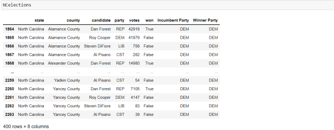
To see the mini data-frame, simply type the name of the mini data-frame you created (NCelections) and run the code. As you can see here, there are 400 records for the North Carolina 2020 gubernatorial elections.

Now, let’s say we wanted to created a new mini data-frame that uses two filtering criteria. Let’s keep the data limited to North Carolina records, but let’s also further filter the data to only display five columns-county, candidate, party, votes, and won.

Here’s the code we’d use:

NCelectionsfiltered = elections.loc[(elections["state"] == "North Carolina"), ["county", "candidate", "party", "votes", "won"]]

Just as with the previous example, we’d use the loc[] function here too. We’d also pass in the elections["state"] == "North Carolina" line as a parameter here too. However, we’d also pass in another parameter-an array of columns that we would like to display in the data-frame; the only columns that will be displayed are those that are included in this list (county, candidate, party, votes, and won in this example). Also remember to separate both of the filtering criteria with a comma.

Now, let’s take a look at the new mini data-frame we created:

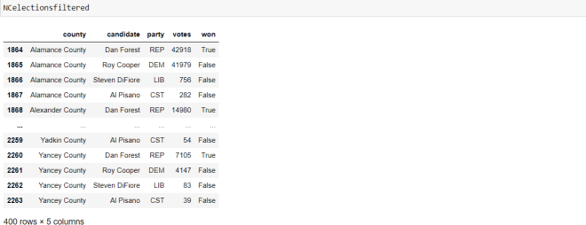
Just like the last mini data-frame we created, this data-frame also has 400 records. However, we only see the five columns we specified in the filtering criteria (which I think makes the data-frame look neater).

The next pandas functionality that I will discuss is grouping data in pandas. A cool thing about pandas data-frames is that they can be split on either rows or columns. You can also group the data by multiple criteria.

Let’s use the original elections data-frame to group the data both by state and by candidate. Here’s how we’d do so:

elections.groupby(["state", "candidate"]).first()

In this example, I used the groupby() function to group the data first by state and then by candidate. To group data in pandas, you’d need to use the groupby() function and pass a list of all the column(s) or row(s) you wish to group the data by as the parameter for this function.

You can also see that I added an additional first() functionality. In this example, first() sorts the data alphabetically, first by state, then by candidate name. In other words, the states are displayed in ascending alphabetical order and the candidates for each state are displayed in ascending alphabetical order by first name (e.g. for Missouri, Jerome Bauer is listed first, then Mike Parson, then Nicole Galloway, and Rick Combs). However, you’ll notice that in the New Hampshire group, Write-ins are displayed before Chris Sununu-this could be because Write-ins aren’t a name and therefore are listed before any of the candidate names.

Next up, I’ll demonstrate how to access individual columns in a pandas data-frame. Let’s say we wanted to access the state, candidate, and party columns (using the original elections dataframe):

elections.loc[:,["state", "candidate", "party"]]

To retrieve specific columns from a data-frame, use the loc[] function and pass in two parameters-: to retrieve the rows from the dataset, and a nested list of column names to retrieve.

Now, regarding the colon (:) parameter-the colon allows you to retrieve all rows of data pertaining to the columns you chose to retrieve. However, if you wanted to only retrieve the first X rows or the last X rows of the dataset, how would you approach this? Let’s see how this would work by retrieving only the first 900 rows:

elections.loc[:899,["state", "candidate", "party"]]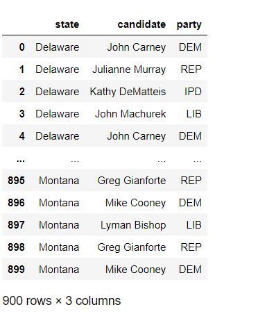

To retrieve the first 900 rows of the dataset, use :899 in place of : as the first parameter of the loc[] function-using :899 tells the loc[] function to only retrieve the first 900 rows of the dataset. If you wanted to retrieve the last 900 rows of this dataset, use 4245: in place of : as the first parameter of the loc[] function.

You’re probably wondering why you’d need to use :899 instead of :900 to retrieve the first 900 rows of the filtered data. This is because the first parameter of the loc[] function involves array indexing, so the first-index-is-0 rule applies here-by that same logic, the 900th index is 899 not 900.

To only retrieve certain columns, you’d need to add a nested list of columns you want to retrieve as the second parameter of the loc[] function-I used the nested list ["state", "candidate", "party"] to retrieve the state, candidate, and party columns.

Next, I’ll show you how to access a certain element in a data-frame. Let’s say we wanted to see how many votes the candidate in the 100th row (index 99) got. Here’s the code we’d use to find the answer to this question (using the elections data-frame):

elections.loc[99].at["votes"]

25647

state                     Indiana
county             Hancock County
candidate            Eric Holcomb
party                         REP
votes                       25647
won                          True
Incumbent Party               REP
Winner Party                  REP
Name: 99, dtype: object

elections.drop(['Incumbent Party', 'Winner Party'], axis=1, inplace=True)

To drop columns in a data-frame, you’ll need to use the drop() function along with three parameters-the column(s) you want to drop, the line axis=1 which signifies that you want to remove a column from a data-frame, and the line inplace=True which ensures that the column will be removed.

It’s important to include the inplace=True line because by doing so, you’ll ensure that you’ll obtain the original data-frame without the removed columns. If you don’t include this line, you’ll simply get a copy of the original data-frame without the removed columns-in other words, the original data-frame with the columns you wanted to remove will still sit in your computer’s memory, which isn’t efficient when dealing with large datasets.

The axis=1 line is also important to include because it signifies that you are removing columns from the data-frame. Using axis=0 would signify that you want to remove rows from the data-frame (I’ll show you how to do this shortly).

• Also, you’ll only need to pass in a list of columns for the first parameter if you’re removing several columns. if you’re only removing a single column, there’s no need to nest that column in a list.

To see the data-frame after removing the columns, simply type the name of the data-frame in your IDE and run the code. Here’s what the elections data-frame looks like after removing the Incumbent Party and Winner Party columns:

Awesome! Now let’s see how to remove rows from a data-frame. More specifically, let’s see how to remove the last row from this data-frame:

elections.drop(5144, axis=0, inplace=True)

Now, let’s see what the elections data-frame looks like (remember to run the line elections on your IDE):

As you can see, the data-frame now has 5,144 rows as opposed to 5,145.

Now, what if you wanted to delete a range of rows as opposed to a single row? Here’s the code we’d use to do so:

elections.drop([0:9], axis=0, inplace=True)

Just like the last example, we’d use the axis=2 and inplace=True values as the second and third parameters, respectively. However, we’d pass an array as the first parameter instead of a single value-the array represents the range of rows we’d like to remove from the dataset.

• I didn’t execute this code-I just included this as an example of how to write your code if you want to remove multiple rows of data.

Now, the cool thing about pandas row-removal is that you can remove rows according to very specific criteria (which you can’t do with columns). Let’s say we wanted to remove all the rows corresponding to Delaware’s gubernatorial elections. How would we do that? Here’s how:

elections.drop(elections.index[(elections["state"] == "Delaware")],axis=0,inplace=True)

In this example, I still used axis=0 and inplace=True as the second and third parameters of the drop function, respectively. However, for the first parameter, I used a nested index() function. Inside the index() function, I passed the filtering criteria I wanted to use to drop rows-elections["state"] == "Delaware". This portion of code lets Python know that I want to drop all rows containing Delaware as the value for state.

Let’s see what the data-frame looks like once we drop the Delaware rows:

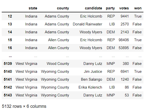
Before we dropped the Delaware rows, there were 5,144 rows in this data-frame. After removing the Delaware rows, we now have 5,132 rows in this data-frame. Interestingly enough, the last index is still 5143-which is what the last index was before we dropped the 5,145th row. Also, since the Delaware rows were also the first 12 rows of the dataset, rows 0-11 have been removed; the first row is the 13th row (or 12th index).

Watch what happens when I try to retrieve row index 8 (the original 9th row):

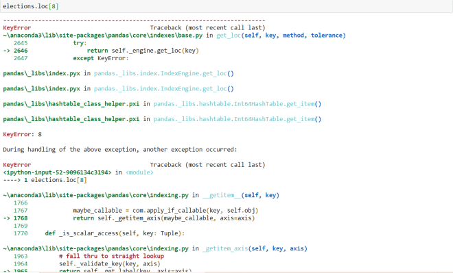
Since row index 8 was deleted, I get an error when trying to retrieve this row index as it no longer exists.

Last but not least, let’s see how to delete a whole data-frame:

del elections

That’s it-it just takes a simple del command to delete a data-frame. Now, let’s try to access the data-frame’s head to see if it’s still there:

As you can see, when we try to access the data-frame’s head after deleting it, we get a NameError telling us that the name elections is not defined. This confirms that the data-frame was successfully deleted.

Thanks for reading,

Michael