Michael here, and today’s post will be a little different than my previous posts. First of all, I know you all are looking forward to more neural network content-and don’t worry, I’ll deliver on that! However, while I get that content ready, I thought I’d do something a little fun for you all by experimenting the popular AI art tool DALL-E 2.
An intro to DALLE 2
We’ll start our journey down the AI art rabbit hole by first discussing the basics of DALLE 2.
First of all, what is DALLE 2? Well, DALLE 2 is the second version of the DALLE AI art algorithm-both DALLE and DALLE 2 were created by OpenAI-the same lab that created the ChatGPT chatbot. In fact, ChatGPT and both iterations of the DALLE art algorithm utilize the GPT (or Generative Pre-Transformer) NLP neural network. The original iteration of DALLE was released in January 2021 and DALLE 2 was released as a beta test in July 2022.
Setting up DALLE 2
Now, how would you start using DALLE 2? First of all, click on this link to be navigated to DALLE’s homepage-https://openai.com/product/dall-e-2:
Once you get to the DALLE 2 homepage, click on the Try DALLE link to start working with DALLE 2. Once you click on this link, you’ll need to sign up for a free DALLE 2 account (if you have a Gmail account, you can simply use these credentials for signing up).
After signing up for a DALLE 2 account, you’ll see a screen that looks like this:
Once you see this screen, you can type a prompt into the text box and have fun creating AI art!
If you haven’t figured out where the name DALLE 2 comes from, it’s simply a portmanteau of the artist Salvador Dali and the PIXAR robot WALL-E (which was a great movie by the way).
You only get 15 free DALLE 2 prompts a month, so use them wisely. Of course, you can always pay for more prompts if you feel inclined to do so-the cheapest deal is 115 prompts for $15 (not bad).
And now let’s create some AI art!
Let’s start with a simple DALLE 2 prompt-perhaps A coloring book page featuring two tabby cats and a ball of yarn. Here’s the output we get:
As you can see, DALLE 2 does quite a great job of creating a coloring book page featuring two tabby cats and a ball of yarn-it even returns one partially colored page.
This prompt, along with any other prompt you type into the input box, will generate four AI art images based off of what you typed into the input box.
Now, let’s try this prompt-A painting of a cow jumping over the moon in the style of Andy Warhol-and see what kind of output we get:
As you can see, DALLE 2 did quite a good job of creating an Andy Warhol-style painting of a cow jumping over the moon. If you’re familiar with Warhol’s work, you’ll be amazed at how well the DALLE 2 algorithm replicates his style (though I would be remiss not to note that DALLE 2’s amazing ability to recreate any art style isn’t without controversy, as this algorithm can easily mimic many art styles without the consent of the artists).
AI art still has a long ways to go
Look, DALLE 2 is smart enough (or rather, built well enough) to generate thousands and thousands of images by working its deep learning magic to mimic thousands of different art styles. But-at least as of March 2023-AI art is still far from perfect.
Let’s say we wanted to generate an AI image of an ice cream shop with the sign Mike's Ice Cream Shop with DALLE 2. Here’s what happens:
In this example, I used the prompt A colored pencil sketch of an ice cream store with a sign that says "Mike's Ice Cream Shop". The four art pieces that were generated create great colored-pencil sketches of an ice cream shops, but none of the storefront signs say “Mike’s Ice Cream Shop”, which is part of the request I sent to DALLE 2. Rather, all the signs generated contain gibberish text (my favorite one is the second picture which has a sign reading “Mik Mic Shke”).
OK, so DALLE 2 can’t really generate a good sign for my made-up ice cream store, but can it generate a good logo for this blog? Let’s find out:
OK, so I asked DALLE 2 to generate a logo for this blog and include the blog’s name-Michael’s Programming Bytes-and its slogan-“Byte sized programming classes for all coding learners”-on the logo. Much like the “Mike’s Ice Cream Shop” example above, the four logos generated don’t contain either the blog’s name or slogan. What the AI-genreated logos contain, however, is a lot of gibberish (though if I ever created a blog called “Mtheglyles” with the slogan “Byilyse”, I’d certainly use the first AI-generated logo).
So, we can see that DALLE 2 isn’t so good with inserting string of text into its AI-generated art. However, can DALLE 2 generate images of people? Let’s find out:
In this example, I typed in the prompt A watercolor painting of President Joe Biden and as you can see from the lack of output above, my request was denied by DALLE 2.
If you click the content policy hyperlink, you’ll be redirected to DALLE 2’s content creation policy, which would give you a better idea as to why this request was denied:
As you can see from the content policy screenshot above, this request was denied because DALLE 2 generally doesn’t accept politically-themed prompts and my Joe Biden prompt fell into that category.
Now, let’s try another prompt that contains a public figure, but this time, let’s make it a non-political public figure. Take a look at the prompt below:
In this example, I used the prompt A photo of a movie poster with Ryan Reynolds' face on it and DALLE 2 generated four images of movie posters with what it thinks is Ryan Reynolds’ face on it. Granted, just like with the ice cream store example, the text on these AI-generated movie posters is pure gibberish, but the face on the first AI-generated poster does resemble Ryan Reynolds pretty closely. The face on the second poster bears somewhat of a resemblance to Reynolds while the third face (and especially the fourth face) looks almost nothing like him.
Interestingly enough, when I swapped Ryan Reynolds’ name (but left the rest of the prompt unchanged) for a female actress-Gal Gadot-this is what I got:
My best guess as to why DALLE 2 will generate images of some public figures (without 100% accuracy) and not others is, aside from their content policy, that OpenAI (the lab that makes DALLE 2) doesn’t want it to be too easy for people to make deepfakes-which in this day and age, would be a fair reason to make it hard to generate fully-accurate images of public figures.
Now that we’ve discovered the limits of DALLE 2 when it comes to generating images of public figures, let’s see how this algorithm does when it comes to generating images of general people:
In this example, I used the prompt A photo of friends on a college campus and the AI-generated results have been quite hit-or-miss. Granted, DALLE 2 did a good job of generating the background-a generic college campus in this case-but DALLE 2 didn’t quite have the same magic when it came to generating images of the people. Let’s take a closer look at one of those images (to take a closer look at an image, simply click on it):
As you can see in this image above, DALLE 2 did a great job of generating the background-a generic college campus-but didn’t do such a good job of generating the generic college students (especially the students’ faces). Also, if you zoom into this picture really closely, you’ll see that the young lady in the orange tank-top has six fingers on one hand.
Yes, even AI has its biases
Aside from DALLE 2’s sometimes imperfect art generations, another thing to note about this algorithm (and AI at large) is that, just like humans, AI has its biases too.
Are you familiar with unconscious bias? If not, it’s a phenomenon that affects how you behave around other people based off of assumptions and/or beliefs you may have about other people just based off of appearances (e.g. baggy clothes, skin color, etc.) rather than their character.
Well, AI does have its unconscious biases too. Think about it-who do you need to create and maintain AI infrastructure? Humans! Since humans have their unconscious biases, they can often incorporate their biases into the programs that they create (though I’m sure this isn’t true for every programmer/developer).
Let’s observe AI bias in action through this DALLE 2 prompt:
So the prompt I used-An oil painting of an American rapper-seems quirky enough, right? Well, take a look at the four AI-generated images and tell me what they have in common. Since all the AI-generated paintings are of black men, this does look like a clear example of unconscious bias in AI.
Let’s try one more example:
OK, so I used the prompt A photo of a kindergarten teacher and surprisingly, got less biased photos than I did in the previous example (but still, 3/4 of the AI-generated photos are of women, and not a ton of diversity in the AI-generated photos).
Interestingly enough, AI seems to fine generating images of people when it’s a single person. When there are multiple people in the picture (as you saw with our college friends example), things fall apart.
Before I go
Before we go, I just want to leave you with some final things I wanted to mention about DALLE 2.
To download any image generated, click on the image itself and once the down arrow icon appears, click on it to download the image:
Also, as per a 2022 ruling by the U.S. Copyright Office, AI-generated images don’t have any copyright protections on them (yet), which means you can use the images as freely as you’d like, but you also can’t claim a copyright on any images you generate through DALLE 2, since after all, the art technically wasn’t created by you but rather by a bunch of 1s and 0s.
Michael here, and today, I thought I’d do something a little different. I won’t be doing any coding projects for today’s lesson, but since I’m currently doing an AI series of blog posts, I though I might take this post to explain the three main types of neural networks you’ll likely encounter in your AI work-CNNs, RNNs and ANNs.
All about ANNs
To begin our post on the three main types of neural networks, let’s first discuss ANNs, or artificial neural networks.
ANNs are the broadest type of neural network, as they encompass basically all types of neural networks. The aim of an ANN is to programaticially mimic the way the human brain thinks using plenty of tiny components that interact with each other-components which are otherwise referred to as artificial neurons (similar to the neurons in a human brain).
In simpler terms, the aim of ANNs is to teach the computer program to do things our brains can do, such as classify images, translate text from one language to another, and even detect people’s faces in an area.
A great example of an ANN can be seen below:
This is the homepage for my YouTube TV account, and above you’ll see a section called TOP PICKS FOR YOU. This is a reccommender section, as it uses an ANN to recommend programs that might be of interest to me based off of my viewing history (as of mid-January 2023). As you can see, the visible part of the TOP PICKS FOR YOU section has lots of cartoons and sports programming.
CNNs-A specific type of ANN
Next up, let’s explore CNNs, or convolutional neural networks, which are a type of ANN.
CNNs are neural networks that are often used for image analysis tasks such as identifying specific people/things in a picture and generating new images/videos from existing images/videos.
How exactly do CNNs work? Well, take a look at this brilliantly-rendered illustration I created on Microsoft Paint in about five minutes:
In this example, the CNN takes the image and utilizes several filtering layers, referred to as convolutional layers, to extract certain features from the image. As you can see from the above picture, this CNN is using four convolutional layers to extract four different features from the photo-face, location (the photo was taken), background (of the photo), and other things in the photo (like the color of my tie).
CNNs often utilize hundreds of convolutional layers-not just four-to extract features from an image.
The convolutional layers then take the details of each feature to generate new images containing these features. The generated images are then passed through multiple pooling layers, which bascially gather the gist of the information from the images generated from the convolutional layers. The CNN then uses fully connected layers to connect the information from both the convolutional layers and the pooling layers to classify objects in images.
Still not getting the gist of how CNNs work? Here’s an example that might help.
If you’ve got photos backed up to Google’s cloud, you’ve likely come across a feature that allows you to locate images based on the people or pets, places, or things that appear in the image. This feature is a great example of CNNs at work, as it uses CNNs to process an image, generate a new image from the original image, and use the information from the new generated image to identify the people, pets, places, or things in the image.
Another type of ANN I wanted to discuss with you is RNNs, or recurrent neural networks. Unlike CNNs, which are mostly used for image analysis tasks, RNNs are used to analyze sequences of data such as text or audio.
How do RNNs work? Well, take a look at my other beautifully-rendered Microsoft Paint illustration to get a visual idea of how RNNs work:
In this example, we’re going to use Taylor Swift music to illustrate how RNNs work. To start the execution of the RNN, we’ll use music from four of Swift’s albums-Reputation, Midnights, Folklore, and Fearless-as input. In this RNN example, each of the albums would be initially processed through an input layer and further processed through a recurrent layer. Each recurrent layer creates connections that allow the information processed from the inputs to flow from one step of processing to the text. How do RNNs accomplish this seamless flow of information? The recurrent layers in RNNs store their “memory”, so to speak, of all the information that was processed from the inputs-the RNN’s “memory” works quite similarly to how our brain’s “memory” works. The RNN’s recurrent layers then use the data gathered from the information processing to generate an output-in this example, the output would be a new AI-generated Taylor Swift song (which, if you’re a Taylor Swift fan, might not enjoy).
Another great example of an RNN would be a chatbot, which is a program that utilizes an RNN to essentially have a conversation with you-a lot of businesses utilize them for customer service matters.
One famous chatbot you’ve likely come across recently is a little tool called ChatGPT, which looks like this:
For those unfamiliar, ChatGPT is a free AI chatbot launched by the AI research lab OpenAI on November 30, 2022. If you have used ChatGPT, you’ll be amazed at how smart and versatile it is. It can do things ranging from writing simple Python scripts (as seen in the screenshot above) to giving you dating advice and…well, the things ChatGPT can do warrants its own blog post (consider this a little preview of future content).
Combining CNNs and RNNs
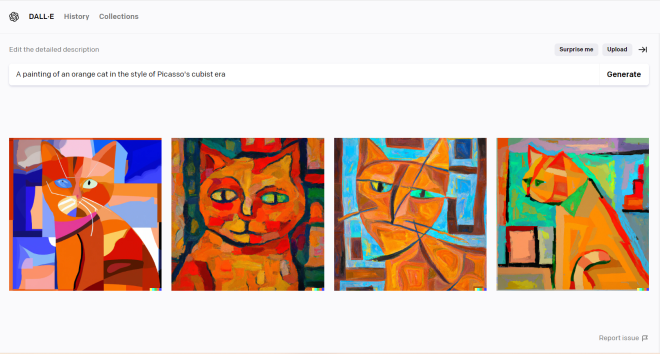
Now, after reading my explinations of CNNs and RNNs, you might be wondering if you can build a tool combining both types of neural networks. The short answer here is yes-and I’ve got a well known example to prove it:
This is a neat, albeit controversial, tool called DALL-E. DALL-E utilizes both CNNs and RNNs to generate pictures based off of a text description. As you can see from the example above, DALL-E did quite a good job of generating a painting of an orange cat in the style of Pablo Picasso’s Cubist era. However, DALL-E’s accuracy in replicating Picasso’s style is also not without its ethical concerns, as it could threaten artists’ livelihoods due to its uncanny accuracy to replicate thousands of art styles.
As for the other things DALL-E can do…well, consider this another preview for a future blog post (because I think DALL-E’s capabilities also warrant its own blog post).
Michael here, and hope you all had a wonderful holiday season. I’ve got lots of exciting content planned for 2023-including something special for the blog’s 5th anniversary (yup, this blog turns 5 on June 13)-and I hope you all will follow along on this programming journey.
To start the year, I thought I’d pick up where I left off in 2022. If you recall, the last post I wrote in 2022 involved creating a basic neural network in Python using the famous MNIST dataset-Python Lesson 38: Building Your First Neural Network (AI pt. 2). In that post, you’ll also likely recall that the neural network we built had an accuracy of less than 20%. In this post, we’ll explore a simple way to improve that neural network’s accuracy. Let’s get coding!
A little refresher on our previous project
In case you’d like to see it again, here’s our code for the neural network project we made in the previous post:
import tensorflow as tf
import keras as kr
import tensorflow_datasets as tfds

(trainX, trainY), (testX, testY) = mnist.load_data()

trainX.shape
testX.shape
trainY.shape
testY.shape

import matplotlib.pyplot as plt
imageNum = 1500
plt.imshow(trainX[imageNum], cmap='magma')

import matplotlib.pyplot as plt
imageNum = 3332
plt.imshow(testX[imageNum], cmap='magma')

firstNeuralNetwork = tf.keras.models.Sequential([
    tf.keras.layers.Flatten(input_shape=(28,28)),
    tf.keras.layers.Dense(150, activation='relu'),
    tf.keras.layers.Dropout(0.2),
    tf.keras.layers.Dense(10)
])

firstNeuralNetwork.compile(optimizer='adam', loss='sparse_categorical_crossentropy', metrics=['accuracy'])
firstNeuralNetwork.fit(x=trainX,y=trainY, epochs=25)

firstNeuralNetwork.evaluate(testX, testY)
To recap, in this code, we built a basic neural network in Python to classify handwritten digits in the MNIST dataset and as I mentioned earlier, this model wasn’t very accurate. In fact, we didn’t acheive accuracy higher than 20% through any of the iterations. Let’s explore some ways we can change that.
One simple way to improve the neural network’s accuracy
Pay attention to this line of code-it creates the second Dense layer in our neural network (the layer that must have ten neurons in this example):
tf.keras.layers.Dense(10)
Similar to what we did for the first Dense layer, add an activation parameter when creating this dense layer (after the number 10). However, this time, set the value of the activation parameter to softmax, like so:
tf.keras.layers.Dense(10, activation='softmax')
You’re likely wondering, what is the softmax function? Here’s an easy way to explain it. Imagine you’re arranging a summertime trip and have four choices of departure dates-June 30, July 1, July 3, and July 5. Let’s say you wanted to use the softmax function to decide a departure date.
The way the softmax function works is that it takes the four aforementioned dates and assigns random probabilities to each of them-the sum of these four probabilites will equal 1 (essentially, we’re dividing the group of possible departure dates into four parts). In this example, let’s say the four probabilities assigned were 46% (for June 30), 20% (for July 1), 19% (for July 3), and 15% (for July 5). All of these probabilites add up to 1-or 100%.
Now that we’ve explained the softmax function, let’s see how it helps improve our neural networks accuracy without changing anything else in the code.
First, let’s see how the accuracy for each epoch is affected:
Well, that’s a significant improvement from the per-epoch accuracy from the previous post! I mean, 77.8% accuracy on just the first epoch is quite impressive-and by the 25th and last epoch-the model achieves 93.7% accuracy.
Now, let’s check out the overall accuracy of the model:
Michael here, and in today’s post-my last post of 2022-I will be showing you how to create your first neural network in Python. I know you haven’t seen stuff like this on my blog before, but I thought I’d end the year teaching you all something new.
Now, there are two possible ways you can create a neural network in Python-one of which involves creating the framework for your neural network by scratch with a combination of classes and functions (which, if you readers want, I’ll cover how to do this). The other way involves using two of Python’s built-in packages-Keras and TensorFlow-which I will discuss more in this post.
A little bit about Keras and Tensorflow
Tensorflow and Keras are two prominent Python neural network machine learning packages. However, Tensorflow is an entire open-source end-to-end neural network package while Keras is more like an interface within Tensorflow. If it helps, think of Keras like a package-within-a-package in Tensorflow; whenever you use Keras, you’re actually using the Tensorflow library. However, Keras is a more intutive version of the Tensorflow libary, albeit with some trade-offs (such as the lack of ability to access more complex functionalities).
Package installation
Before we get started with our neural network creation, let’s first install our packages. You’re going to need both Tensorflow and Keras for this tutorial, but you only need to run the pip install tensorflow command on the command prompt, as installing Tensorflow will usually install Keras too. However, on the off chance that Keras doesn’t get installed with Tensorflow, you could run the pip install keras command on the command prompt.
Just in case you forgot, if you want to check if you’ve already pip-installed a certain package, run the pip list command and run through the list of installed packages to find the package you’re looking for (all packages are listed in alphabetical order).
Setting up the neural network
For this lesson, we’re going to start off by building a simple neural network-one that works with the MNIST Keras dataset. For those who don’t know, the MNIST (Modified National Institute of Standards and Technology) dataset is a very, very large dataset of images containing the handwritten digits 0-9-the MNIST dataset is commonly used for training image processing systems (or if you’re just starting out with neural network machine learning). This dataset contains 70,000 28×28 pixel images-60,000 images for the training dataset and 10,000 images for the testing dataset.
The MNIST dataset is certainly larger than most of the other datasets we’ve worked with in earlier posts (if you recall, the datasets from my earlier machine learning posts had about a few thousand elements tops). The reason for this is because, unlike the other machine learning I’ve taught you (k-means clustering, Naive Bayes classifications), neural networks are really well-suited for large datasets-and by large, I mean at least 10,000 records.
To start creating our neural network, first include these three lines of code in your Jupyter notebook:
import tensorflow as tf
import keras as kr
import tensorflow_datasets as tfds
Pay attention to the highlighted import line-in addition to the Tensorflow and Keras packages, you’ll also need the tensorflow_datasets package for this lesson. The tensorflow_datasets package contains several Tensorflow datasets you can work with when developing neural networks (such as the MNIST dataset, which we will be working with in this lesson).
If you haven’t installed the tensorflow_datasets package yet, run the line pip install tensorflow_datasets on your command prompt or run the line !pip install tensorflow_datasets on your Jupyter notebook (or whichever IDE you’re using).
Loading the MNIST dataset (and a word of advice)
Now that we’ve imported the necessary packages into our Python IDE, the next thing we need to do is import the MNIST dataset into our IDE. Here’s the code to do so:
from keras.datasets import mnist
Unlike most of my other machine learning/data analytics posts, I won’t be attaching a dataset to this post because we’ll be using a built-in Python dataset for this post. If you’re familiar with some popular data analytics/machine learning datasets such as titanic (detailing survivors and victims of the Titanic disaster), iris (detailing petal and sepal widths of a sample of 50 irises), and mtcars (detailing various features about a bunch of old cars), you’ve probably seen them on A LOT of data analytics/machine learning tutorials. There’s a good reason for that-they’re freely available and built-in datasets on several programs (Python and R to name just two).
For those who’ve been following my blog for a while, you’ll notice that I try to stay away from overly cliche datasets (I mean, if you’re a data science/data anayltics machine learning student, you’re probably quite sick of the iris dataset). However, even though MNIST is a very commonly used (and a little cliche) dataset, I think it will be the most appropriate first dataset to introduce you all to neural network creation.
Also, final word of advice for you all-if you’re trying to build a data science/data analytics/machine learning portfolio to land yourself a tech job (as I did when I launched this blog in summer 2018), try to stay away from cliche datasets. Find datasets that stand out (and ideally interest you)-you’ll be sure to impress the recruiters!
Now back to the lesson! After importing the MNIST dataset into your IDE, run this line of code to split the MNIST dataset into training and testing datasets:
When loading the MNIST dataset into your IDE (or any large dataset for that matter), remember to split your dataset into training and testing datasets, each denoted by their own variables.
I know it’s been a while since I’ve done any machine learning posts, so as a refresher, when building a machine learning model, the training dataset trains the model to work while the testing dataset is used to test if the model works as intended. When working with machine learning datasets, don’t split the main dataset 50-50 into training and testing datasets. The training dataset should be the larger dataset; a split like 70% training/30% testing should work fine-though the MNIST dataset has a split of ~85% training/~15% testing, which will work for this dataset.
Why do we need X and Y training and testing datasets? The X datasets encompass the whole dimensions of the training and testing datasets-the size (60,000 for training and 10,000 for testing) along with the dimensions of each image (28×28 pixels). The Y datasets on the other hand just encompass the sizes of each dataset.
In case you’re wondering about the size of each X and Y dataset, run the .shape command for each like so-remember not to include a pair of parentheses after each .shape command, as you can’t call tuple objects:
Now that we’ve loaded our MNIST dataset into Python, split the data into training and testing datasets, and obtained the shapes of each dataset, it’s time to get our feet wet and build our first neural network!
However, before we dive into the neural network nitty-gritty, there’s something I want to show you. Take a look at the code and output below:
import matplotlib.pyplot as plt
imageNum = 1500
plt.imshow(trainX[imageNum], cmap='magma')
In this example, I imported the matplotlib.pyplot package (which you may recall from my MATPLOTLIB lessons) to plot the 1501st image in the MNIST training dataset in MATPLOTLIB’s magma color scheme (the cmap parameter refers to MATPLOTLIB’s color schemes). As you can see, this image of a handwritten 9 is displayed as a 28×28 pixel image-which makes sense, as all images in the MNIST dataset (both training and testing) have a 28×28 pixel size.
In order to plot any of the images in the MNIST dataset, you’ll need to use either of the X datasets (in this example, trainX and testX) since they encompass the image sizes and in turn, contain the actual images. The Y datasets simply encompass the images themselves, so you would be able to retrieve any element from the MNIST dataset from either of the Y datasets, but you won’t be able to plot the image itself.
Just like many of the other Python projects I’ve done throughout this blog involving lists, the MNIST dataset is basically a giant zero-indexed list of images. So for a parameter like imageNum, you can choose any value between 0 and 59,999 if you’re analyzing the 60,000 image training dataset. If you’re analyzing the 10,000 image testing dataset, you can choose any value between 0 and 9,999. In the example above, I chose the 1,501st image in the testing dataset (as the imageNum I chose was 1,500, which represents the element at index 1,500).
Just for fun, let’s also plot a random image from the testing dataset:
import matplotlib.pyplot as plt
imageNum = 3332
plt.imshow(testX[imageNum], cmap='magma')
In this example, I did the same thing as I did in the previous example, except I decided to plot the 3,333rd image from the MNIST testing dataset-which happens to be the number 4.
Now that we know how to plot each element in the MNIST dataset (for both the testing and training datasets) it’s time to create our model! Take a look at the code below to see how we can create our first Python neural network model:
Now, if you’ve never seen a Python neural network before, you’re probably wondering what all of this code means. But don’t worry-your friendly neighborhood coding blogger is here to break it all down for you!
First off, let’s start with the Sequential sub-module. We use this sub-module in order to create the outer part of the neural network; in this sub-module, we wrap all the functions for the neural network inside of a list wrapped inside of the Sequential object constructor (referrring to the pair of parentheses that enclose the list). Why do we need a sequential model for the neural network? In this example, using a sequential model for the neural network allows us to add the other four layers in this neural network-Flatten, Dense, Dropout, and Dense-in sequential order, which is important for neural networks.
Now what about the four layers wrapped in our sequential model-Flatten, Dropout and the two Dense layers? The Flatten layer, well, flattens the input from 2-dimensional to 1-dimensional-which is important as we’re dealing with thousands of 2-D images for this dataset. How does Flatten flatten the input data? The Flatten layer’s input_shape parameter takes in the dimensions of the object to flatten-in this case each 28×28 image in the MNIST dataset-and takes in the (28, 28) tuple as the value of the input_shape argument.
The Dropout layer removes some of the data from the model in order to prevent overfitting. In the context of machine learning, what is overfitting? Overfitting in machine learning is what happens when your model has excellent accuracy with training data but not with new and unfamiliar data.
Let me give you an example. Let’s say you want to create a model that predicts whether an employee at a very, very, very large company is going to get a promotion based off of their resume. Let’s also assume that you train a model containing 5,000 resumes and it predicts outcomes with 96% accuracy-pretty awesome, right! Now let’s say you feed the model a new set of 2,500 resumes and it predicts outcomes with only a 44% accuracy-what happened here? The model experienced overfitting, as it was able to predict outcomes with great accuracy for the training dataset but with less-than-stellar accuracy for the new and unfamiliar dataset.
In our neural network, the Dropout layer will ignore 10% of the data in the training dataset to avoid overfitting.
Last but not least, we have two Dense layers for our neural network. The first Dense layer activates the neural network using the ReLU, or rectified linear unit activation, function. For more on the algebra behind ReLU, check out this article-https://machinelearningmastery.com/rectified-linear-activation-function-for-deep-learning-neural-networks/ (if you’re into linear algebra and/or trigonometry, I think you’ll enjoy this article). In the most basic sense, ReLU is a linear activation function that is used in a lot of neural networks due to its easy-to-train and well-performance.
In the first Dense layer, you’ll notice a number right before the activation parameter-that number indicates how many neurons you want to have in the neural network upon activation; in this case, we have 150 neurons upon activation of our neural network. The second Dense layer also has a number too-10. What’s the difference between these two numbers? In the first Dense layer, you can have as many neurons as you’d like upon activation while in the second Dense layer, you must have 10 neurons as there are ten unique objects for classifcation (images of the numbers 0-9).
Fitting and Compiling the Model
The last two things we need to do before we deploy our model are to fit it and compile it. How can we do that? Take a look at the code below:
So, what does all of this code mean? First of all, the optimizer parameter and value set the neural network’s optimization alogrithm-in this case, we’re using Tensorflow’s adam optimizer (for a more in-depth explination on that optimizer, check out this link-https://www.educba.com/tensorflow-adam-optimizer/), though you can experiement with whatever Tensorflow optimizer you like.
The loss parameter and corresponding value set the neural network’s loss function, which is used to help optimize the model’s performance by measuring the discrepancies between the predicted values and the target values. In the context of the MNIST dataset, each element would be considered a target value and the value that the neural network predicts as part of its classification would be the target value. In this example, we’re using the sparse_categorical_crossentropy loss function, which measures the cross-entropy (or contrast or discrepancy) between the predicted values and the actual values.
The metrics parameter and corresponding value (or list in this case) set the metrics-or in this case, metric-that you’d like to use to measure the neural network’s accuracy. In this example, we’re going with the accuracy metric, as this is the easiest metric to understand. Accuracy is also often used as a baseline for other metrics such as precision and f1 score (which is similar to accuracy but it takes false positives and false negatives into account).
In the fit function, you’ll first need to pass in your training datasets for both the X and Y values. As for the epoch parameter and value, an epoch is essentially an iteration through all the training data that isn’t ignored by the Dropout layer. To train a neural network and optimize it for accuracy, iterating through all of the training data once won’t suffice-you’ll need at least 10 iterations through the training data to optimize your neural network (though more epochs couldn’t hurt). In this neural network, we’re using 25 epochs, meaning that we will iterate through the training data 25 times.
Now, let’s see how our neural network performs through each epoch (or iteration):
In this epoch run log, we can see several different metrics for each epoch, such as loss and accuracy. However, the only metric you should focus on is each epoch’s accuracy, as that tells you the accuracy of the neural network throughout each training run. For instance, the first epoch (denoted as Epoch 1/25) had an accuracy of 11.18%. The final epoch (denoted as Epoch 25/25) had an accuracy of 11.17%-all in all, pretty abysmal accruacy for the neural network.
Neural network evaluation time!
Last but not least, it’s neural network evaluation time! To evaluate the accuracy of the overall model (as opposed to individual epochs), all you need is one line of code:
Just like you saw with the epochs, you’ll see the loss and accuracy metrics. Pay close attention to the accuracy metric, as this will tell you the model’s overall accuracy, which is still pretty bad at 10.45%.
I know this may seem confusing, but remember when you’re fitting & compiling the model to use the training dataset (for both the X and Y axes). When you’re evaluating the model’s accuracy, use the testing dataset (for both the X and Y axes).
Yes, I know the accuracy of this neural network sucked. However, the aim of this lesson was not to build the best neural network out there-rather, my aim was to teach you the basics of neural network creation so that you all knew the basic concepts of neural networks. A lot of the concepts we discussed in this post-activation algorithms, epochs, dropout rate-can be experimented with to your liking in order to optimize the neural network’s accuracy.
Final code and some parting words for 2022
So, I know we had A LOT of code for this lesson. In case you wanted to run the code in the order we discussed it, here’s the entire script below for your convinience (outputs not included):
import tensorflow as tf
import keras as kr
import tensorflow_datasets as tfds
(trainX, trainY), (testX, testY) = mnist.load_data()
trainX.shape
testX.shape
trainY.shape
testY.shape
import matplotlib.pyplot as plt
imageNum = 1500
plt.imshow(trainX[imageNum], cmap='magma')
import matplotlib.pyplot as plt
imageNum = 3332
plt.imshow(testX[imageNum], cmap='magma')
firstNeuralNetwork = tf.keras.models.Sequential([
    tf.keras.layers.Flatten(input_shape=(28,28)),
    tf.keras.layers.Dense(150, activation='relu'),
    tf.keras.layers.Dropout(0.2),
    tf.keras.layers.Dense(10)
])
firstNeuralNetwork.compile(optimizer='adam', loss='sparse_categorical_crossentropy', metrics=['accuracy'])
firstNeuralNetwork.fit(x=trainX,y=trainY, epochs=25)
firstNeuralNetwork.evaluate(testX, testY)
Thanks for coming along on this coding journey in 2022! Hope you all sharpened your skills and/or learned something new along the way this year! Have a very happy holiday season and rest assured-I will be back in 2023 with brand new coding content (and a little something special for my blog’s 5th anniversary)!