It’s Michael here, and today’s lesson will be on cleaning a pandas data-frame (pt.3 in my pandas series).
Analyzing data certainly gives you useful insights on your data-however, most real life datasets don’t look as neat as the datasets we’ve worked with over the course of this blog’s run. Oftentimes, real life datasets can be quite messy, which means you’d need to tidy them up before working with them.
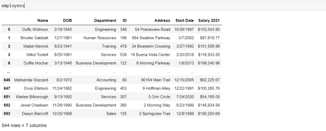
Here’s the messy dataset we’ll be working with in this post:
This datasets contains data regarding 650 employees at a company. And in case you’re wondering, unlike with most of my blog posts, this data doesn’t pertain to anything in real life. I completely made it up.
Now, let’s open up our IDE, import the pandas package, and read our data-frame into our IDE:
import pandas as pd

employees = pd.read_csv('C:/Users/mof39/OneDrive/Documents/Employee data.csv')
Keep in mind that the dataset I’m using and the dataset I provided for you guys have different names-that’s because WordPress doesn’t let me upload CSVs and the read_csv function doesn’t work with XLSX files. The dataset I provided for you guys and the dataset I’m using in this code is the same dataset-just named differently so I can easily distinguish between the CSV and XLSX files.
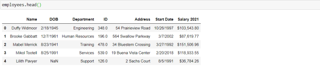
Great! Now, let’s take a look at the head of our data-frame:
As you can see, our dataset has seven variables. Let’s explore what each variable represents:
Name-The name of the employee
DOB-The employee’s date of birth
Department-The employee’s department in the company
ID-The employee’s employee ID number
Address-The employee’s home address
Start Date-The date the employee started with the company
Salary 2021-The employee’s base (pre-tax) salary for the calendar year 2021.
However, we can’t yet create any visualizations with this data or conduct any meaningful analyses. Here are the things we must clean up first:
Two employee records are repeated multiple times.
There are several null records in the DOB column.
Several records in the ID column are stored as float, not int.
First, let’s take care of the null records in the DOB column. When dealing with null/blank records in a data-frame, there are two ways you can deal with this issue:
Remove the rows with null values from the dataset.
Replace the null values with a specific value or the mean/median/mode of the values in the column.
Well, since the null records are found in a date column, replacing the nulls with the mean/median/mode won’t work here. We could replace the null records in the DOB column with something like 1/1/2021 or we could remove the rows with null records altogether.
In this case, let’s remove the null records altogether. Here’s the code to do so:
employees.dropna(inplace=True)
You will only need a single line of code with the dropna() function in order to drop all null rows from the dataset. Now, you’re probably wondering what inplace=True means-this line of code signifies that you want to drop all null rows from your current data-frame. If you don’t include this line of code, a new data-frame with the null rows removed will be created-your current data-frame (employees) won’t be changed at all.
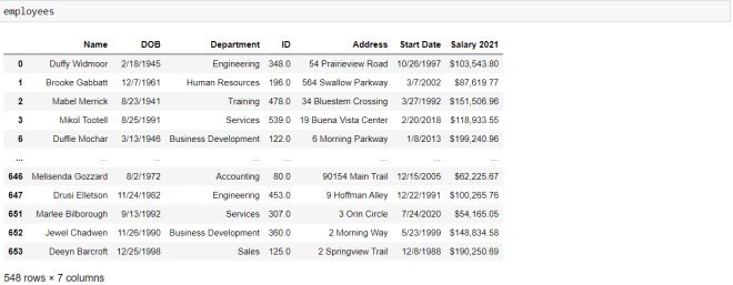
Now, let’s see what the dataset looks like without the null rows:
As you can see, there are now 548 rows in the dataset (there were 654 rows before we removed the null records).
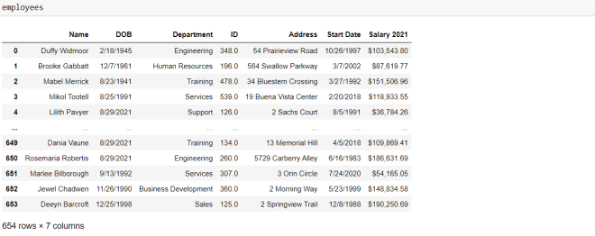
But what if you didn’t want to remove all the records with null birthdates? What if you simply wanted to fill all null DOB records with a placeholder date-let’s say 8/29/2021. Here’s the code you’d need to run:
To replace all the null values in a certain column with a placeholder value, use the fillna() function with two parameters-the value you’d want to use to replace the null values and the inplace=True line. The inplace=True line works the same way here as it does with the dropna() function.
Another thing to note is that if you only want to replace the null values in a specific column, you’d need to specify that column before the fillna() function. If you don’t do this, ALL null values in the data-frame will be replaced, which isn’t ideal since the values in each column of your data-frame are usually of different data types.
Now, the second bit of cleaning we’d need to do is to change the ID values to type int-they are currently of type float. Here’s the code we’d use to change the data type of values in a pandas data-frame column:
To change the data type of the values in the ID column from floats to integers, use the to_numeric() function and pass in two parameters-the column that you want to format (employees["ID"]) in this case and downcast=integer. The reason for the downcast=integer line is to ensure all of the values in the ID column will be converted into integers. Had we not included this line, the data type of the values in the ID column would’ve still been floats.
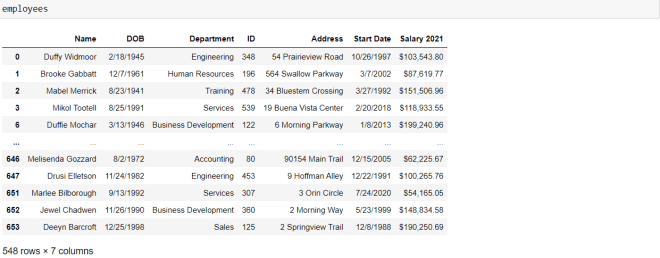
Now, let’s see what the table looks like after this modification:
As you can see, all of the values of the ID column are now integers.
Note, this is what the data-frame looks like after I dropped the null DOB values, not after I filled the null DOB values with 8/29/2021.
Last but not least, I mentioned that two employees’ records are duplicated. Let’s see how we can remove duplicate values from a data-frame:
employees.drop_duplicates(inplace=True)
To remove the duplicates from the data-frame, simply use the drop_duplicates() function and pass in the parameter inplace=True.
Last but not least, let’s export our cleaned data-frame to a CSV file. Here’s the code to do so:
employees.to_csv('C:/Users/mof39/OneDrive/Documents/Employee data cleaned.csv')
After specifying the data-frame you want to export, use the to_csv() function to export the data-frame. You’ll need to pass in 1 parameter-the location on your computer where you want to store the cleaned data frame. It’s that simple.
Michael here, and today’s lesson will cover more pandas Python fundamentals-this is the second lesson in my pandas series.
Now that I’ve introduced you all to the basics of Python’s pandas package, let’s discover some more fundamental functionalities of the Python pandas package.
The dataset I’ll be using is the 2020 US gubernatorial election dataset I used in the previous post. Here’s the link to that post, where you will find that dataset: Python Lesson 24: The Basics of Pandas (pandas pt. 1).
Before we begin, be sure you have the pandas package installed on your computer. Once you confirm that you have the pandas package installed, run these two lines of code:
import pandas as pd

elections = pd.read_csv('C:/Users/mof39/OneDrive/Documents/2020 Gubernatorial Data.csv')
The first line of code will import the pandas package to Jupyter Notebook (or whatever IDE you’re using). The second line of code will read the 2020 Gubernatorial Data CSV file to your IDE.
The downloadable dataset actually comes in an XLSX format, but that’s only because WordPress wouldn’t let me upload CSV files. However, you’ll need a CSV file for the second line of code to work. An easy workaround would be to change the .XLSX at the end of the file name to a .CSV, which automatically changes the file type to a CSV.
Now, before we begin exploring some other basic pandas functionalities, let’s explore each of the variables in this dataset, as I feel it will be important to do so for context:
state-the state where the election took place
county-the county in a particular state
candidate-the gubernatorial candidate on the ballot in a particular state’s election
party-the political party of the candidate
votes-how many votes the candidate earned in a particular county
won-whether the candidate won the gubernatorial election in a state (True means they won and False means they lost)
Incumbent Party-the political party of the state’s incumbent governor (as of November 2020)
Winner Party-the political party of the winner of the state’s gubernatorial election (effective January 2021)
Great, now that we’ve explained the data and created the data-frame, let’s start exploring more pandas functionalities!
The first thing I’ll demonstrate is how to create a smaller data-frame from a larger data-frame (slicing a data-frame, in other words). Let’s say we wanted to create a smaller data-frame that focuses on the North Carolina 2020 gubernatorial election. How would we do so? Here’s how:
To slice a pandas data-frame, use the loc[] function. Notice that you’ll need to pass in parameters into square brackets rather than the regular parentheses.
Speaking of parameters, you’ll need to pass in the filtering criteria that you will use to create your new array-you’ll also need to pass in the filtering criteria in regular parentheses ().
Pay attention to the filtering criterion I used-elections["state"] == "North Carolina". In this section of code, I’m specifying that I want to create a new data-frame containing only records from the original data-frame (elections) where the state is North Carolina.
The loc[] function is always appended to the name of the original data-frame (e.g. elections.loc[(...)].
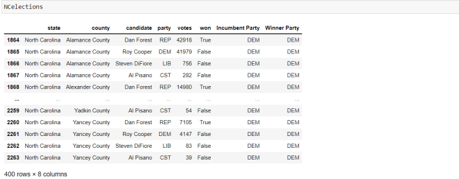
Now, let’s take a look at the new mini data-frame we created:
To see the mini data-frame, simply type the name of the mini data-frame you created (NCelections) and run the code. As you can see here, there are 400 records for the North Carolina 2020 gubernatorial elections.
Now, let’s say we wanted to created a new mini data-frame that uses two filtering criteria. Let’s keep the data limited to North Carolina records, but let’s also further filter the data to only display five columns-county, candidate, party, votes, and won.
Just as with the previous example, we’d use the loc[] function here too. We’d also pass in the elections["state"] == "North Carolina" line as a parameter here too. However, we’d also pass in another parameter-an array of columns that we would like to display in the data-frame; the only columns that will be displayed are those that are included in this list (county, candidate, party, votes, and won in this example). Also remember to separate both of the filtering criteria with a comma.
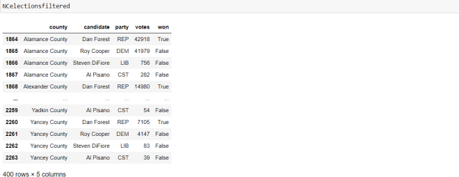
Now, let’s take a look at the new mini data-frame we created:
Just like the last mini data-frame we created, this data-frame also has 400 records. However, we only see the five columns we specified in the filtering criteria (which I think makes the data-frame look neater).
The next pandas functionality that I will discuss is grouping data in pandas. A cool thing about pandas data-frames is that they can be split on either rows or columns. You can also group the data by multiple criteria.
Let’s use the original elections data-frame to group the data both by state and by candidate. Here’s how we’d do so:
elections.groupby(["state", "candidate"]).first()
In this example, I used the groupby() function to group the data first by state and then by candidate. To group data in pandas, you’d need to use the groupby() function and pass a list of all the column(s) or row(s) you wish to group the data by as the parameter for this function.
You can also see that I added an additional first() functionality. In this example, first() sorts the data alphabetically, first by state, then by candidate name. In other words, the states are displayed in ascending alphabetical order and the candidates for each state are displayed in ascending alphabetical order by first name (e.g. for Missouri, Jerome Bauer is listed first, then Mike Parson, then Nicole Galloway, and Rick Combs). However, you’ll notice that in the New Hampshire group, Write-ins are displayed before Chris Sununu-this could be because Write-ins aren’t a name and therefore are listed before any of the candidate names.
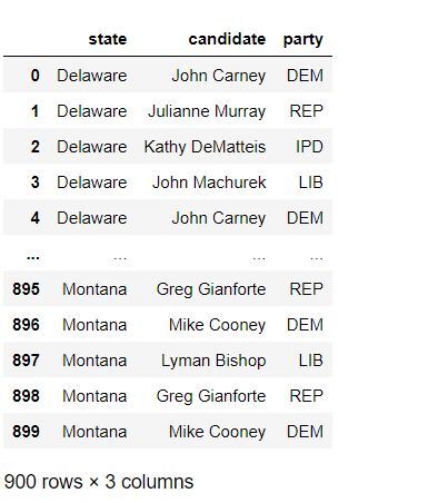
Next up, I’ll demonstrate how to access individual columns in a pandas data-frame. Let’s say we wanted to access the state, candidate, and party columns (using the original elections dataframe):
elections.loc[:,["state", "candidate", "party"]]
To retrieve specific columns from a data-frame, use the loc[] function and pass in two parameters-: to retrieve the rows from the dataset, and a nested list of column names to retrieve.
Now, regarding the colon (:) parameter-the colon allows you to retrieve all rows of data pertaining to the columns you chose to retrieve. However, if you wanted to only retrieve the first X rows or the last X rows of the dataset, how would you approach this? Let’s see how this would work by retrieving only the first 900 rows:
To retrieve the first 900 rows of the dataset, use :899 in place of : as the first parameter of the loc[] function-using :899 tells the loc[] function to only retrieve the first 900 rows of the dataset. If you wanted to retrieve the last 900 rows of this dataset, use 4245: in place of : as the first parameter of the loc[] function.
You’re probably wondering why you’d need to use :899 instead of :900 to retrieve the first 900 rows of the filtered data. This is because the first parameter of the loc[] function involves array indexing, so the first-index-is-0 rule applies here-by that same logic, the 900th index is 899 not 900.
To only retrieve certain columns, you’d need to add a nested list of columns you want to retrieve as the second parameter of the loc[] function-I used the nested list ["state", "candidate", "party"] to retrieve the state, candidate, and party columns.
Next, I’ll show you how to access a certain element in a data-frame. Let’s say we wanted to see how many votes the candidate in the 100th row (index 99) got. Here’s the code we’d use to find the answer to this question (using the elections data-frame):
elections.loc[99].at["votes"]

25647
So how did we get 25,647 as the output? Let’s break down this code function-by-function. The first function, elections.loc[99], returns this pandas object:
state                     Indiana
county             Hancock County
candidate            Eric Holcomb
party                         REP
votes                       25647
won                          True
Incumbent Party               REP
Winner Party                  REP
Name: 99, dtype: object
When using the loc[] function to retrieve an element from a pandas data-frame, the number that you pass into the loc[] parameter corresponds to the row that will be returned. Since I passed in 99 as the loc[] parameter, the function will retrieve the 100th row in the elections data-frame (loc[99] corresponds to the 100th row).
The second function in the above code-.at["votes"]-retrieves the value of the votes column that corresponds to the 100th row in the elections data-frame. Since the values of votes for the 100th row is 25,647, 25,647 is the output for the function.
The last thing I will show you is how to delete columns & rows from a data-frame. Let’s say we wanted to remove the Incumbent Party and Winner Party columns. Here’s the code we’d use to do so:
To drop columns in a data-frame, you’ll need to use the drop() function along with three parameters-the column(s) you want to drop, the line axis=1 which signifies that you want to remove a column from a data-frame, and the line inplace=True which ensures that the column will be removed.
It’s important to include the inplace=True line because by doing so, you’ll ensure that you’ll obtain the original data-frame without the removed columns. If you don’t include this line, you’ll simply get a copy of the original data-frame without the removed columns-in other words, the original data-frame with the columns you wanted to remove will still sit in your computer’s memory, which isn’t efficient when dealing with large datasets.
The axis=1 line is also important to include because it signifies that you are removing columns from the data-frame. Using axis=0 would signify that you want to remove rows from the data-frame (I’ll show you how to do this shortly).
Also, you’ll only need to pass in a list of columns for the first parameter if you’re removing several columns. if you’re only removing a single column, there’s no need to nest that column in a list.
To see the data-frame after removing the columns, simply type the name of the data-frame in your IDE and run the code. Here’s what the elections data-frame looks like after removing the Incumbent Party and Winner Party columns:
Awesome! Now let’s see how to remove rows from a data-frame. More specifically, let’s see how to remove the last row from this data-frame:
elections.drop(5144, axis=0, inplace=True)
Since there are 5,145 rows in this data-frame, you’d pass in 5144 as the first parameter since 5144 corresponds to the index of the last row of data. Similar to the previous example, right? However, you’d pass in axis=0 as the second parameter of the drop() function rather than axis=1 because you’re removing a row, not a column. You’d also include the inplace=True argument to signify that you want to return the original data-frame with the dropped row rather than a copy of the data-frame with the dropped row.
Now, let’s see what the elections data-frame looks like (remember to run the line elections on your IDE):
As you can see, the data-frame now has 5,144 rows as opposed to 5,145.
Now, what if you wanted to delete a range of rows as opposed to a single row? Here’s the code we’d use to do so:
elections.drop([0:9], axis=0, inplace=True)
Just like the last example, we’d use the axis=2 and inplace=True values as the second and third parameters, respectively. However, we’d pass an array as the first parameter instead of a single value-the array represents the range of rows we’d like to remove from the dataset.
I didn’t execute this code-I just included this as an example of how to write your code if you want to remove multiple rows of data.
Now, the cool thing about pandas row-removal is that you can remove rows according to very specific criteria (which you can’t do with columns). Let’s say we wanted to remove all the rows corresponding to Delaware’s gubernatorial elections. How would we do that? Here’s how:
In this example, I still used axis=0 and inplace=True as the second and third parameters of the drop function, respectively. However, for the first parameter, I used a nested index() function. Inside the index() function, I passed the filtering criteria I wanted to use to drop rows-elections["state"] == "Delaware". This portion of code lets Python know that I want to drop all rows containing Delaware as the value for state.
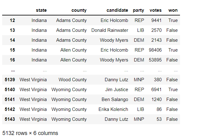
Let’s see what the data-frame looks like once we drop the Delaware rows:
Before we dropped the Delaware rows, there were 5,144 rows in this data-frame. After removing the Delaware rows, we now have 5,132 rows in this data-frame. Interestingly enough, the last index is still 5143-which is what the last index was before we dropped the 5,145th row. Also, since the Delaware rows were also the first 12 rows of the dataset, rows 0-11 have been removed; the first row is the 13th row (or 12th index).
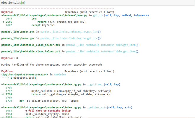
Watch what happens when I try to retrieve row index 8 (the original 9th row):
Since row index 8 was deleted, I get an error when trying to retrieve this row index as it no longer exists.
Last but not least, let’s see how to delete a whole data-frame:
del elections
That’s it-it just takes a simple del command to delete a data-frame. Now, let’s try to access the data-frame’s head to see if it’s still there:
As you can see, when we try to access the data-frame’s head after deleting it, we get a NameError telling us that the name elections is not defined. This confirms that the data-frame was successfully deleted.
Michael here, and today’s post will be a Python lesson that demonstrates the basics of the pandas package-this will be the first lesson in my pandas Python series.
So, what does the pandas package do? Well, just like the NumPy package, pandas is another package for working with datasets in Python. However, one major difference between the pandas and NumPy packages is that pandas has functions to read data into Python, while NumPy has no such functionality (yet). The pandas package is also better suited for cleaning up messy data sets than the NumPy package.
To use the pandas packages, run the pip install pandas command on your command prompt (or better yet, before you run this command, run pip list on the command prompt to see if pandas is already installed and if it isn’t, then run the pip install pandas command).
In this case, I already have the pandas package installed on my computer, so no need to install it again.
After you’ve installed the pandas package on your computer, run the import pandas as pd command to import pandas onto whatever Python IDE you are using (I’m using Jupyter notebook for these posts).
Great! Now that we’ve gotten the installation underway, let’s start exploring some of the basic things we can do with the pandas package.
One of the most common things that you can do with pandas is read CSV files into Python. Here’s how to do so:
In this line of code, I read a CSV dataset stored on my computer onto Python using the pd.read_csv function. This dataset contains data on various 2020 gubernatorial elections that occurred in the United States (I was going to use this for a blog post last year but never did). You should also save your dataset as a variable, which represents a pandas data frame.
As you all might have figured out, to read a CSV dataset into pandas, you’d need to use the pd.read_csv() function and pass in the path to the CSV file as this function’s parameter.
If your CSV file is stored in the same directory where you’re running this code, simply passing in the name of the CSV file will work (though don’t forget to add the .csv at the end of the file name.
Passing in an XLS or XLSX file won’t work here!
Now that we’ve read the dataset into Python, let’s do some exploratory analysis!
First, let’s see what the head of the dataset looks like:
The head of the dataset refers to the first X rows of the dataset. You can specify a number in the head() function parameter, but if you don’t, the first five rows of the dataset will be displayed be default.
When displaying the head of the dataset, use this syntax-dataframe name.head(rows to display)
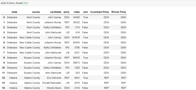
Ok, what if we wanted to see this dataset’s first 10 rows? Here’s how we’d execute the code:
To display the first 15 rows of the data-frame, I ran the code elections.head(15)-passing in 15 as the parameter of the head() function.
Now that we’ve learned to display the head of the dataset, let’s display the tail of the dataset. In case you didn’t figure out the head/tail logic-the head refers to the first X rows of the dataset while the tail refers to the last X rows of the dataset.
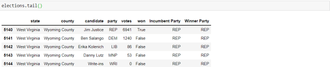
Here’s how to display the tail of the dataset:
To display the tail of a dataset, you’d use the same syntax that you’d use to display the head of a dataset, except you’d swap the head() function for the tail() function. Also, just as with the head() function, you can pass in a number for the tail() function and if you don’t pass in a number, the last five rows will be displayed by default (recall that with the head() function, if you don’t pass in a number into the function, the first five rows will be displayed by default.
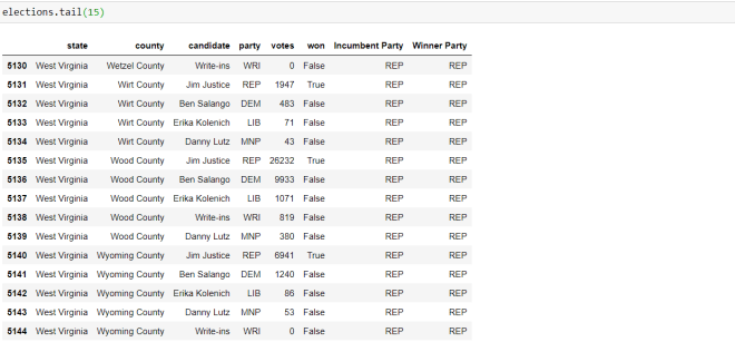
Now, let’s display the last 15 rows of the dataset:
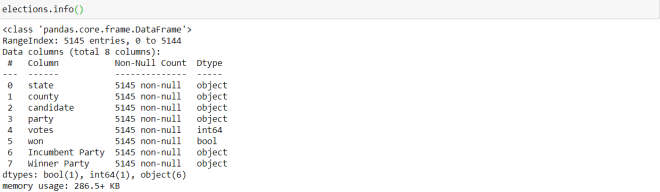
Now, what if we wanted to retrieve the basic information about this dataset? The info() function allows us to do just that:
The syntax to run the info() function is name of dataframe.info(). Unlike the head() and tail() functions, you can’t pass in any parameters to the info() function.
The info() function displays the following information:
The class of the elections object (a pandas.core.frame.DataFrame)
The RangeIndex (which indicates the number of records in the dataset-5145)
The names of each of the variables/columns, the non-null count (which shows how many non-null records are in a certain column) for each column, and each columns’ variable type
The dtypes and count of each dtype (which simply displays a count of each variable type in the dataset)
Michael here, and today’s lesson will be on using views and copies in NumPy arrays-this is part 6 in my NumPy series.
What exactly are copies and views in NumPy? Copies and views are both replications of a NumPy array, but with some major differences. A copy is a new array that’s created from a replication of another array while a view is simply a replication of an array rather than a new array entirely. A copy and the original array are stored in different locations in a computer’s memory while a view and the original array are stored in the same memory location.
Another major difference between NumPy copies and views is that copies own the original array’s data, thus, any changes made to a copy won’t affect the original array. On the other hands, views don’t own the original array’s data, thus, any changes made to a view will affect the original array.
In both examples, I modified the duplicate array (A in both examples) to replace the second element with 144. As you can see, in the copy example, 24 was replaced with 144 in the duplicate array but not in the original array. In the view example, 24 was replaced with 144 in both the duplicate array and original array.
Now, how can you find out if a replicated array is a copy or view? Take a look at this example:
To find out if an array is a copy or a view, use the .base attribute alongside the duplicated array. If the array is a copy, None will be returned. If the array is a view, the original array (numpyA in this example) will be returned.
In order for the np.concatenate function to work properly, you’d need to pass in all the arrays you’d like to concatenate into a single tuple; if you pass in the arrays one-by-one, the function won’t work.
Also, when you concatenate multiple NumPy arrays, the dimensions stay the same:
Numpy1 and numpy2 are both 1-D arrays; the combined array numpy3 is also a 1-D array.
Now, can we join two arrays with different dimensions together? Let’s take a look:
numpy4 = np.array([[3, 6, 9], [4, 8, 12]])
numpy5 = np.array([5, 10, 15])
numpy6 = np.concatenate((numpy4, numpy5))
print(numpy6)

---------------------------------------------------------------------------
ValueError                                Traceback (most recent call last)
<ipython-input-14-479431df35d4> in <module>
      1 numpy4 = np.array([[3, 6, 9], [4, 8, 12]])
      2 numpy5 = np.array([5, 10, 15])
----> 3 numpy6 = np.concatenate((numpy4, numpy5))
      4 print(numpy6)

<__array_function__ internals> in concatenate(*args, **kwargs)

ValueError: all the input arrays must have same number of dimensions, but the array at index 0 has 2 dimension(s) and the array at index 1 has 1 dimension(s)
As you can see, trying to concatenate two arrays with different dimensions doesn’t work; all of the arrays you’re trying to concatenate must have the same number of dimensions.
Now, in the array concatenation examples I’ve shown you, the arrays are being joined along the same axis. How could you join arrays along different axes?
You would stack the arrays together. Here’s an example of NumPy array stacking:
Stacking arrays is the same as concatenation, except stacking is usually done along a new axis. To stack a NumPy array, use the np.stack function and pass a tuple containing the arrays you want to stack and the axis you want to stack them on; if you don’t pass an axis into np.stack, arrays will automatically be stacked along the first axis.
What would it look like if these arrays were stacked along the first axis rather than the second axis? Take a look:
All of the elements from both arrays will still be present, however, stacking along the first axis creates a 2×3 array, while stacking along the second axis creates a 3×2 array. Both stacked arrays are still 2-D.
In case you didn’t figure it out, axis=0 refers to the first axis while axis=1 refers to the second axis.
You can’t stack along a non-existent axis; in this example, the stacked array only has two dimensions, therefore you can’t stack along axis=2 because the stacked array has no third dimension and thus has no third axis.
Stacking along axes works well, but what are some other NumPy array stacking methods?
Let’s say you wanted to stack along rows. Here’s how to do so:
To stack an array along rows, use the np.hstack function and pass in a tuple containing the arrays you want to stack. In this example, stacking along rows simply merged the two arrays into a single 1-D array with the elements of numpy7 being listed before numpy8.
Now what if you wanted to stack along columns? Here’s how to do so:
To stack arrays along columns, use the np.vstack function-the parameter for this function is the same as the parameter for the np.hstack function (a tuple containing the arrays you want to stack). In the example, stacking along columns created a 2×3 2-D array (this is the same outcome as stacking along the first axis).
Now, there’s another way that you can stack your array-along depth (or height). Here’s how to do so:
Stacking along depth/height is the same gist as stacking along rows or columns-the only difference is that you’d use the np.dstack function to stack along depth/height. In this example, stacking along depth/height created a 3×2 3-D array, which is interesting because in the example where I stacked along the 2nd axis in a previous example (using the same three NumPy arrays), I got a 3×2 2-D array.
Now that we’ve discussed the basics of joining NumPy arrays, let’s discover how to do the reverse (splitting arrays).
Here’s a simple example of splitting a NumPy array:
To split up a NumPy array, use the np.array_split function and pass in two parameters-the array you want to split up and the number of splits you want to use on the array. In this example, I have an array of 10 elements that I split in two.
Something to note when splitting areas is that the number of splits you want to use on an array doesn’t need to be divisible by the number of elements in the array. Granted, I did use two splits on a 10-element array. Watch what happens when I use three splits on the same 10-element array:
Accessing individual arrays from a larger split NumPy array is the same as accessing elements from an individual array-in this case, the first array is index 0, the second array is index 1, and so on.
Now what if we wanted to access individual elements from these split arrays? Take a look at this example:
To access an individual element in each individual array, you’d need to add another indexing call. In this example, the first indexing call refers to the array itself while the second indexing call refers to the element inside the array.
Now, how would you split a multi-dimensional array? Take a look at this example:
In this example, I am splitting a 2-D array in two-interestingly enough, both of the split arrays are still 2-D.
As you can see in the example, there are two 1-D arrays inside the 2-D array, therefore, splitting the 2-D array in two made sense. However, what if you wanted to split this 2-D array another way? Let’s see what happens when we split this array in three:
When you split this array in three, you get both of the 1-D arrays in the 2-D arrays plus a blank array with a shape of (0, 6). If I was to split this array in four, I would’ve gotten both of the 1-D arrays plus two blank arrays with a shape of (0, 6).
A neat thing about splitting arrays is that, just like with joining arrays, you can split the arrays along a certain axis. Let’s see how axis-splitting an array works with a 2-D array:
In this example, I split the 2-D array numpy14 in five, resulting in a split array where elements from both of the 1-D arrays are stacked on top of each other in two columns. To split a NumPy array along a certain axis, specify the axis you want to split along after the number of splits you want to perform.
Just as with axis-joining an array, if you don’t specify an axis to split along in the np.array_split function, the array will automatically split along the first axis.
You can’t split along an axis beyond the scope of the array. In this example, since numpy14 is a 2-D array, you can’t split along axis=2 since a 2-D array doesn’t have a third axis.
Now, I mentioned that you can join arrays along rows, columns, and depth/height. However, did you know that each of the array-joining functions-np.hstack, np.vstack, and np.dstack-also have array-splitting counterparts-np.hsplit, np.vsplit, np.dsplit?
Let’s demonstrate the np.hsplit function first, which splits your array along rows:
In this example, I split numpy16 in two along rows; as you can see, both split arrays are displayed along a single row. Also, even though np.hsplit is the counterpart to np.hstack, np.hsplit doesn’t require a tuple as a parameter since you’re splitting a single array rather than stacking multiple arrays on top of each other.
Now let’s check out the np.vsplit function, which splits your array along columns:
Interestingly, the output for np.vsplit is displayed in the same format as the output for np.hsplit. However, keep in mind that unlike for np.hsplit, np.vsplit won’t work on 1-D arrays-you’ll need at least a 2-D array to make np.vsplit work.
Finally, let’s demonstrate the np.dsplit function, which splits your array along depth/height:
Unlike the output for np.hsplit and np.vsplit, the output for np.dsplit displays stacked, with elements from each 1-D array interspersed with each other. Also, for np.dsplit to work, you’ll need at least a 3-D array; 2-D arrays won’t work with np.dsplit.
Turns out, accessing elements from a 2-D array is simple as well, except you’d use two parameters rather than just one. The first parameter specifies which dimension you’d like to search in and the second parameter specifies the element in that dimension you’d like to retrieve. In this example, I’m retrieving the third element from the first dimension (recall that Python arrays have an indexing system that starts with 0).
Simple enough right? Now let’s see how we can access elements from a 3-D array:
This one is a bit more complex since there is more to break down, but there’s an easy way to explain 3-D array indexing. First of all, since there are three dimensions, there are obviously three parameters you’d need to use.
Aside from that, the first parameter is 1, which tells Python to look for an element in the second dimension. The second parameter is 2, which narrows the search down to the third array within the second dimension. The third parameter is 1, which further narrows down the search to the second element within the third array within the second dimension-the element that is returned from this search is 44.
Now let’s demonstrate how to perform negative (or reverse) indexing on a 1-D array:
Reverse indexing on a NumPy array is the same as reverse indexing on a regular Python array. In this example, I am retrieving the element at index -2 (1.2), which refers to the second index from the right of the array.
Now here’s reverse indexing at work on a multi-dimensional array:
Reverse indexing on a multi-dimensional array is also fairly simple. In this example, I am retrieving the last element (or rightmost element) from the second array-within-an-array.
One more neat thing about NumPy array indexing is that it allows you to perform basic arithmetic on certain elements of the array. Here’s an example of that:
In this example, I am performing the four basic arithmetic operations (addition, multiplication, subtraction, and division) and exponentiation (raising a number to a certain power) on certain elements in the array; I’m using different elements for each operation.
Next up, let’s discuss slicing an array. In the context of programming, array slicing is when you take certain element(s)/portion(s) from an array to create a new, smaller array. Here’s a simple example of NumPy array slicing:
In this example, Python is printing out the first five elements of arrG. Recall that when retrieving a range of elements from an array, the element corresponding to the end index is not included-so in this case, the 6th element wasn’t included.
Now, just as with regular Python arrays, you can slice arrays without a start index or end index-you just need one of these indexes to slice an array. Let me show you what I’m talking about:
print(arrG[5:])

[2002 2006 2010 2014 2018 2022]
In this example, I used [5:] to retrieve the sixth element in the array onward.
print(arrG[:5])

[1982 1986 1990 1994 1998]
In this example, I used [:5] to retrieve all elements in the array up to BUT NOT INCLUDING the sixth element.
The next topic I want to discuss is negative (or reverse) slicing; just as you can perform reverse indexing on an array, you can also perform reverse slicing on an array as well.
Let me show you an example of reverse slicing:
print(arrG[-4:-1])

[2010 2014 2018]
Reverse slicing has the same idea as reverse indexing-indexing starts at -1, which corresponds to the rightmost element in the array (2022 in the case of arrG).
If I wanted to include 2022 in my reverse slicing, I would’ve used this code:
print(arrG[-4:])

[2010 2014 2018 2022]
Had I used the line print(arrG[-4:0]), I would’ve recieved an empty array as output.
Now let’s explore a new array concept that I haven’t discussed here before-the concept of step. The step concept allows you to set a step for the slicing (e.g. return every other element, etc.).
Let’s see a simple example of slicing an array by step:
print(arrG[::3])

[1982 1994 2006 2018]
In this example, I retrieved every third element from arrG starting with the first element-1982. In other words, I retrieved the 1st, 4th, 7th, and 10th elements from arrG.
Now what if I wanted to perform step slicing only on a certain portion of the array:
print(arrG[0:6:2])

[1982 1990 1998]
In this example, I am performing step slicing on the 1st-7th elements of arrG (which correspond to indexes 0-6) by retrieving every other element from this portion of the array. If you want to perform step slicing on a portion of the array (rather than the whole array), you need to specify the portion of the array you would like to slice in the first two parameters-in this example, since I wanted to perform my slicing on elements 1-7, I used 0 and 6 as the first two parameters in the above example.
Now, how would we slice multi-dimensional arrays? Here’s an example (using a 2-D array):
In this example, the slicing function (referring to the line arrH[0, 1:4]) has two parameters rather than one-the first parameter contains the dimension where you wish to perform the slicing and the second parameter contains the range of elements you would like to retrieve (up to but not including the end index).
In the slicing function, I retrieved the 2nd through 4th elements (indexes 1-4) in the first dimension of the array (index 0). Step slicing also works for multi-dimensional arrays; for instance, the line print(arrH[0, ::2]) would have worked here (and it would have returned the 1st, 3rd, and 5th elements from the 1st dimension).
Now, how would we go about slicing a 3-D array? Take a look at the example below:
In order to slice a 3-D array, you’d need 3 parameters for the slicing function-the first parameter represents the 2-D array within the 3-D array where you wish to perform the slicing, the second parameter represents narrows the slicing focus to a 1-D array within the 2-D array you selected, and the third parameter represents the range of elements in the 1-D array that you want to retrieve.
In this example, the first parameter is 0, which tells Python to start the array slicing in the first (and only) 2-D array within the 3-D array. The next parameter is 1, which tells Python to narrow the array slicing focus to the second 1-D array within the 2-D array. The last parameter is 0:3, which tells Python to retrieve the 1st-3rd elements from the second 1-D array within the 2-D array.
Last but not least, let’s explore how to iterate through NumPy arrays (which involves looping through all array elements).
To iterate through NumPy arrays, a for loop while do the trick. Here’s an example of iterating through a 1-D array:
for x in arrJ:
    print(x)

10
15
20
25
30
35
40
45
50
55
60
65
70
To iterate through a simple 1-D array, all you need is the lines for x in [array name]: print(x). Not hard at all.
Let me discuss the arange function I used. The arange function is simply another way to create a NumPy array; this function has 4 parameters-the first element in the array, the last element in the array, the increment/decrement that is used to generate each element of the array, and the number type of the elements in the array (you usually use int or float).
Now let’s demonstrate iterating through a 2-D array:
Looks good right? The for loop syntax I used might work if you want to iterate through each 1-D array but this doesn’t work if you want to iterate through each element (known in programming lingo as a scalar) in each array-within-an-array.
Here’s how to iterate through each 1-D array in the 2-D array:
for x in arrK:
    for y in x:
        print(y)

1
1
2
3
5
8
13
21
34
55
89
144
A simple way to iterate through multi-dimensional arrays is the use of nested for loops. In this example, the outer for loop iterates through the main 2-D array while the inner for loop iterates through each element in each 1-D array within the 2-D array.
This is a great way to iterate through multi-dimensional arrays, but here’s an even better way to iterate through multi-dimensional arrays:
for x in np.nditer(arrK):
    print(x)

1
1
2
3
5
8
13
21
34
55
89
144
Simply using NumPy’s nditer function (and passing your array as a parameter) will iterate through each element in your array with just a simple line of code. The nditer function is super helpful because it allows you to iterate through a multi-dimensional array with a single line of code; recall that NumPy arrays can go up to 32-D, which would make for a very cumbersome-to-write nested for loop.
Now check out the two methods when used for iterating through a 3-D array. Which do you think is more efficient?
arrL = np.array([[[2, 4, 8, 16, 32], [3, 9, 27, 81, 243], [4, 16, 64, 256, 1024]]])

for x in arrL:
    for y in x:
        for z in y:
            print(z)

2
4
8
16
32
3
9
27
81
243
4
16
64
256
1024
for x in np.nditer(arrL):
    print(x)

2
4
8
16
32
3
9
27
81
243
4
16
64
256
1024
As you can see, both methods work great for iterating through arrL. However, the nditer method is more efficient and accomplishes the iterating with one line of code (the nested for loops method uses three lines of code).
Finally, I wanted to discuss step iterating through an array. Just as you can perform step slicing on an array, you can also step iterate through an array too:
for x in np.nditer(arrL[:, ::3]):
    print(x)

2
4
8
16
32
In this example, I am iterating through arrL but only returning every third element.
For step slicing and step iteration, remember that the step starts with the first element in the array unless you specify otherwise!
In this example, I created a 2-D array with six elements in each array. To find out the array’s shape, I called the array’s .shape function. The shape is shown as (2, 6), which means that this array has 2 dimensions and 6 elements per dimension.
Now how would we reshape this array? Let’s say that we wanted to turn this 2-D array into a 3-D array. Here’s how we would do that:
To reshape a NumPy array, use the .reshape function on your current array and change the parameters of the .reshape function to the dimensions you want the new array to have.
In this example, I changed the shape of arrayA to 3 X 4, which means that the new array (stored in the arrayB variable) will have 3 dimensions with 4 elements in each dimension.
Look, the .reshape function is quite versatile, but you can just use any two numbers as the parameters here. Here’s what happened when I tried reshaping arrayA to 5×7:
Since 5 and 7 aren’t factors of 12 (the array size), Python couldn’t reshape the array to 5×7.
In order to know all of the possible ways that you can shape the array, count all of the elements in the array (12 in the case of arrayA) then make a note of all of the factors of that amount. Since there are 12 elements in arrayA, the possible shapes arrayA can take include (1, 12), (2, 6), and (3, 4), as these are all number pairs that have a product of 12.
(12, 1), (6, 2), and (4, 3) work as well-recall that, from the Commutative Property of Multiplication, you can switch the order of the factors around and get the same product. However, keep in mind that the dimensions will be different if you switch the order of the numbers.
Also, when reshaping the array, keep in mind that dimensions are capped at size 32 (I mentioned this in the previous lesson)
Now I’ve demonstrated how to reshape a NumPy array with a standard number-pair tuple. However, did you know that you can also include an unknown dimension. Here’s how that works:
Yes, NumPy allows you to use -1 as a shape parameter in the .reshape method. But what does this mean? -1 simply represents an unknown dimension that you want NumPy to figure out. How does NumPy figure out this unknown dimension? It looks at the length of the array and the known dimension(s) in order to determine how to best shape the array. In this example, NumPy sees that the known dimension is 2, so the array is shaped to have two rows with five elements per row-the array has 10 elements, so 10 divided by 2 (# of rows) equals 5 (# of elements per row).
Now what if I had switched the order of the parameters in the .reshape function to (-1, 2). What would we get?
If I switch the order of the .reshape function parameters to (-1, 2), the array would still have 10 elements but instead of 2 rows-by-5 columns, I get an array with 5 rows-by-2 columns.
As you can see, using the unknown dimension trick of -1 works just great with two shape parameters. However, the -1 trick also works with three shape parameters. Take a look at the example below:
In this example, using -1 as the second shape parameter still splits the array in two, except you get two 1×5 arrays.
You can only have one unknown dimension in every .reshape function!
For all of the known dimensions, you can only include factors of the array length. In other words, since arrayD has a length of 10, you could only use 1, 2, 5, or 10 for the known dimension(s), as these are all the factors of 10.
The next NumPy trick I will show you is how to flatten arrays. In NumPy, you can convert multi-dimensional arrays into 1-D arrays-this is called flattening the array-with a simple line of code. Here’s how to flatten a NumPy array:
To flatten a NumPy array, simply use the .reshape function with the -1 parameter. That’s it. However, for the flattening to work, only use the -1 shape parameter-don’t include other shape parameters!
Now I know I said that the array-flattening trick works with multi-dimensional arrays, but it also works with 0-D arrays. Here’s an example of this:
As you can see, my 0-D was successfully turned into a 1-D array.
Last but not least, I want to show you two special NumPy functions that you will likely encounter if you’re learning about more advanced Python topics (e.g. computer vision)-.zeros and .ones. These functions allow you to create arrays of zeros and ones, respectively (recall that 0 and 1 are the two elements in the binary number system from Java Lesson 5: Java Numbering Systems).
In this .zeros function, I used two parameters-a tuple to specify the shape of the array (4×4) and a value to specify the type to store the zeros (int).
Let’s say I didn’t specify a value type for the zeros. How would they be stored on the program?
In this example, I didn’t set a value type for the zeros, so they are by default stored as type float64-which is a 64-bit floating point number.
If you want to check the type of all the values used in the NumPy array, use the .dtype function, not .type.
The number of shape parameters you use for the shape tuple in the .zeros and .ones functions indicates the number of dimensions your array will have. In the example above, I used two shape parameters for the shape tuple, therefore my array has two dimensions.
Michael here, and today’s Python lesson will be a little different than the Python lessons we’ve done before. Now that I’ve covered some of the basic building blocks of Python, I figured it’s time to dive into some cooler stuff (e.g. data analytics, natural language processing, etc.) that you can do with Python. Right now, I’ll start with diving into the data analytics side of Python.
Now, let’s get started with learning the basics of one of Python’s most basic data analytics packages-NumPy. NumPy is a special Python package that is used for working with numerical arrays-NumPy is actually short for “numerical Python”.
However, to use NumPy, you need to be sure that it’s installed on your computer. To install a Python package to your computer, you would need to pip install the package on your computer’s command prompt like so:
If you’re wondering what pip is, it’s the package that Python uses to install other packages (think of pip as Python’s main package manager). Oftentimes, pip will already come installed with whatever Python IDE you chose to use (I use both Jupyter Notebook and Anaconda in my development), but in case it isn’t, here’s the link to download pip onto your computer-https://pypi.org/project/pip/.
To install the NumPy package, simply type this line onto your command prompt-pip install numpy. Sometimes, there are certain packages already pip installed on your laptop, so you’ll get a message on the command prompt that says Requirement already satisfied:, as I did above (apparently NumPy was already pip installed on my computer).
If you wanted to uninstall NumPy (or any other Python package), simply type pip uninstall numpy (you can replace this with any other python package you pip installed) onto the command prompt. The pip package manager will then ask you if you want to uninstall the python package.
You don’t have to pip install Python packages in any particular directory, but I’d recommend that you perform any pip installs in your main directory (the directory with the structure “C:/Users/[your username]”)
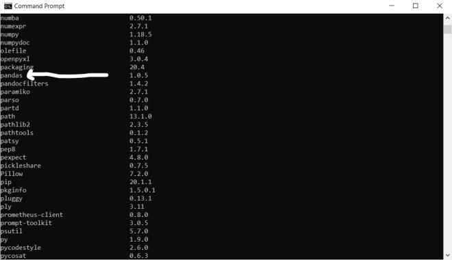
Now, if you wanted to see a list of all the Python packages that are installed on your computer (along with the corresponding versions of each package), type pip list onto the command prompt like so:
As you can see, I have numpy version 1.18.5 installed on my computer.
Depending on the Python library you need for your project, running pip list can help save you a pip install.
Now that I’ve covered all the pip install material, let’s dive right in to NumPy!
To use NumPy in your IDE, first run this line of code-import numpy as np. The as np part is completely optional since np is simply the alias for numpy. Including the as np part in your import statement allows you to refer to the NumPy package as np rather than numpy (in other words, as np is just convenient shorthand for NumPy).
Now here’s an example on how to create a simple NumPy array:
To create a NumPy array, simply use the np.array() function and use an array-like object as the parameter for this function. In this example, I used the list [2, 4, 6, 8, 10] as the parameter for the np.array() function.
For your information, NumPy arrays are stored with the type ndarray.
Now, I did mention that you can use an array-like object as the parameter for the np.array() function. Lists aren’t the only parameter accepted by this function; tuples work great too. Here’s an example of using a tuple in the np.array() function:
In this example, the tuple I passed into the np.array() function is converted into a NumPy array (of type ndarray). The magic of the np.array() function is that it can convert any array-like object (like a list or a tuple) into a NumPy array.
Pretty cool stuff right? Now, did you know that you can create multi-dimensional arrays, which are arrays with extra levels of array depth. Put simply, multi-dimensional arrays can contain any number of nested arrays, which are arrays within arrays.
Here’s how to make a 0-D (0-dimensional) array:
array3 = np.array(50)

print(array3)

50
Looks simple right? 0-dimensional arrays consist of a single element. That’s it.
Now, if you want to know to create a 1-D array, refer to the examples with array1 and array2, as these are two excellent examples of 1-D NumPy arrays. 1-D arrays consist of array-like objects (like lists or tuples) as their elements.
Now here’s an example of how to create a 2-D array:
In this example, I created a 2-D array by wrapping a list of three 1-D arrays inside a pair of square brackets ([]). As for the ndim call, it simply shows you how many dimensions are in a NumPy array (2 in this case).
Now here’s an example of how to create a 3-D array:
A NumPy 3-D array consists of several 2-D arrays; each 2-D array in the 3-D array is printed on a separate line, as you can see above.
Getting the brackets right for 3-D arrays does get tricky, so keep that in mind.
Now I’ve shown you how to create 0-D, 1-D, 2-D, and 3-D arrays. However, NumPy arrays aren’t limited to a 3-dimension maximum; the sky’s the limit when it comes to the amount of dimensions a NumPy array can have.
Let’s say we wanted to create a 6-dimensional NumPy array. How would we go about doing that? Take a look at the code below:
To add X number of dimensions to a NumPy array, simply create a 1-D array and specify the number of dimensions you want in the array using the ndmin parameter.
As you can see, since I created a 6-dimensional array in the above example, there are six pairs of square brackets surrounding the array. Just for fun, let’s see what happens when we create a 50-dimensional array (using the same elements as array6):
As you can see, that didn’t work. Apparently NumPy arrays can only have 32 dimensions tops. Even an experienced Python coder like me learns something new everyday.
Michael here, and today’s lesson will be on performing date & time manipulation in Python. Now I know I did a date & time manipulation lesson in R (check out R Lesson 19: Fun With Dates & Times), but I want to show you how it’s done in Python.
Before I get started with any coding examples, I think it will be important to mention that dates aren’t data types. However, we can import a datetime module to create date & time objects; to import the datetime module, use the line import datetime.
Now, here’s how to use the datetime module to display the current date and time:
now = datetime.datetime.now()

print(now)

2021-04-15 22:16:45.356841
In this example, I created a datetime object-now-that displays the current date and time (using the 24-hour format for time) using the datetime.now() method of the datetime module. Simple enough, right?
Well, along with displaying the current date & time, the datetime module also has several format codes to retrieve information about a datetime object. Let’s say we wanted to retrieve the current month (fully spelled out) and the current day of the week (in shorthand). Here’s how to do so:
now = datetime.datetime.now()

print(now.strftime("%a"))
print(now.strftime("%B"))

Thu
April
In this example, I am retrieving the current day of the week (in shorthand) and the current month (fully spelled out) from the current datetime-April 15, 2021 10:16:45PM. To retrieve the shorthand day of the week, I used the format code %a and to retrieve the fully spelled out month, I used the format code %B. Also, in order to use these format codes, I need to use them as parameters in the function strftime.
Here’s a list of all the format codes you can use with the strftime function (all examples refer to the now object):
%a-returns the shorthand version of the weekday.
example: %a would return Thu (which is shorthand for Thursday)
%A-returns the fully spelled out version of the weekday
example: %A would return Thursday (the name of the weekday spelled out)
%w-returns the corresponding number of the weekday; the weekdays are numbered from 0-6, with 0 being Sunday and 6 being Saturday
example: %w would return 4 (Thursday corresponds to 4)
%d-returns the day of the month (which can range from 01-31)
example: %d would return 15 (the day of the month in the now object is 15)
%b-returns the shorthand version of the month
example: %b would return Apr since the month for the now object is April.
%B-returns the fully spelled out version of the month
example: %B would return April (which is the month for the now object)
%m-returns the number of the month (which can range from 01 to 12):
example: %m would return 04 since April is the 4th month of the year
%y-returns the last two digits of the year:
example: %y would return 21 since the year is 2021
%Y-returns the full version of the year:
example: %Y would return 2021 since the year is 2021
%H-returns the hour according to a 24-hour clock:
example: %H would return 22 since the time is 10:16 PM.
%I-returns the hour according to a 12-hour clock:
example: %I would return 10 since the time is 10:16 PM.
%p-returns AM or PM depending on whether the time is before or after 12 noon.
example: %p would return PM since the time is 10:16 PM.
%M-returns the minute of the time part of the datetime object (ranging from 00-59)
example: %M would return 16 since the minute of the time part of now is 16.
%S-returns the second of the time part of the datetime object (ranging from 00-59)
example: %S would return 45 since the second of the time part of now is 45 (the full time is 10:16:45 PM)
%f-returns the millisecond part of the datetime object (ranging from 000000-999999)
example: %f would return 356841 since the millisecond part of now is 356841 (the full time with milliseconds is 10:16:45.356841 PM)
%z-returns the difference between the current time and UTC time (in hours)
example: I know I didn’t set a time-zone for now, but if I did, %z would return -0600 since I’m writing this post from the US Central Time Zone and US CST is 6 hours behind UTC.
%Z-returns the time-zone
example: %Z would return CST as I’m currently in the US Central Time Zone (this would work if I had set a time zone)
%j-returns the day number of the year (ranging from 001-366)
example: %j would return 105 as April 15 is the 105th day of the year.
An important thing to note here is that if the date for now was set to April 15, 2020, %j would return 106 since April 15 is the 106th day of the year in leap years.
%U-returns the week number of the year (ranging from 00-53); this format code assumes weeks start on Sunday
example: %U would return 20 as April 15, 2021 falls on the 20th week of the year 2021.
The %U format code would return 01 for January 3-9, 2021, as this is the first full week of the year. However, for January 1-2, 2021, %U returns 00. Interestingly, for December 27-31, 2020 (which falls on the same week as January 1-2, 2021), %U would return 52.
%W-returns the week number of the year (ranging from 00-53); unlike the format code %U, this format code assumes weeks start on Monday
example: %W would also return 20 since it is still the 20th week of the year 2021 (even though %W uses the weeks-starting-on-Monday system)
%c-returns the local date and time; the local date and time is displayed using this format-(day of week) (month & day) (local time in 24-hour format) (year)
example: %c would return Thu Apr 15 22:16:45 2021 as that is the local time stored in the now object.
Only the hours, minutes, and seconds are returned from the local time.
%x-returns the date in mm/dd/yy format
example: %x would return 04/15/21
%X-returns the local time in 24-hour format
example: %X would return 22:16:45
Just as with regex special sequences, the letter casing can be very easy to mix up between format codes, so keep that in mind.
Date format codes start with percent signs while regex special sequences start with backslashes (it can be very easy to confuse date format codes with regex special sequences).
Now, what if I wanted to create my own datetime object? Here’s how to do so:
In this example, I created my datetime object date1 and set the parameters equal to 2021, 4, and 18, respectively. When I printed the date1 object, I got the output 2021-04-18 00:00:00.
How did I get this output? Well, since I used 2021, 4, and 18 as parameters, I got the date 2021-04-18 since the year is the first parameter to set when creating a datetime object followed by the month and day.
However, you’re probably wondering how I got the time 00:00:00. See, when I create a datetime object, I can not only set a date but I can also set a time. Aside from the year, month, and day, I can also set an hour, minute, second, millisecond, and time zone parameter. All of these parameters are optional when creating a datetime object, and if no value is specified for each of these parameters, 00 is the default value-hence why the outputted time was 00:00:00.
Now that I’ve shown you the basic things you can do with the datetime package, let’s discuss how to perform date manipulation.
First of all, what if we wanted to calculate the difference between two dates? Here’s how we would do so:
date2 = datetime.datetime(2021, 9, 9)
date3 = datetime.datetime.now()
delta = date2 - date3

print("There are" ,delta.days, "more days until the 2021 NFL season.")
There are 143 more days until the 2021 NFL season.
In this example, I created two datetime objects-date2 and date3-and created a variable delta to determine the difference between the two dates.
Just so you know, the date being referenced in now is April 18, 2021. Also, the 2021 NFL season starts on September 9, 2021, hence why the date2 parameters are (2021, 9, 9).
After subtracting the two datetime objects, I then get the message There are 143 more days until the 2021 NFL season. Just for reference, here is the print statement I used: print("There are" ,delta.days, "more days until the 2021 NFL season."). The delta.days statement returns the number of days between the two datetime objects.
Now, what if you wanted to find the amount of weeks between two dates? Here’s how to do so:
date2 = datetime.datetime(2021, 9, 9)
date3 = datetime.datetime(2021, 4, 18)
delta = date2 - date3

print("There are" ,round(delta.days/7, 1), "more weeks until the 2021 NFL season.")

There are 20.6 more weeks until the 2021 NFL season.
Unfortunately, finding the number of weeks between two dates isn’t as simple as using delta.weeks (I know because I tried this). If you want to find the amount of weeks between two dates, simply divide the result of delta.days by 7. The decimal generated by delta.days/7 is quite long, so it’s often useful to round the decimal (using the round function) to either 1 or 2 decimal places as I did above.
Now let’s see how we can get the amount of months between two dates:
date2 = datetime.datetime(2021, 9, 9)
date3 = datetime.datetime(2021, 4, 18)
delta = date2 - date3

print("There are" ,round(delta.days/30, 1), "more months until the 2021 NFL season.")

There are 4.8 more months until the 2021 NFL season.
In this example, I used the same approach to finding the amount of months between two dates as I did when I was trying to find the amount of weeks between two dates (even rounding the quotient to one decimal place). The only difference between this example and the previous example is that I divided delta.days by 30 to find the amount of months between the two dates.
You probably guessed this, but there is no delta.months function. Hence why we need to divide the result of delta.days by 30.
In order to get the amount of months between two dates, you don’t have to divide delta.days by 30. 28 might work, but when I tried dividing delta.days by 28 in the above example, I got 5.1 (I felt that 4.8 was more accurate).
Now I’ve shown you how to create datetime objects as well as calculate the difference (in days, weeks, and months) between two datetime objects. What if we wanted to find out the date that would be X days before or after a certain date? Here’s how to do so:
In order to add or subtract days from a certain date, I would first need to import the timedelta module from the datetime package (use the line from datetime import timedelta). In this example, I created a datetime object date4 and set it to the current date & time (April 19, 2021 at 10:10 PM). I then created a newdate object and set it equal to the value of date4 plus 20 days from date4 using the timedelta(days=20) function-I then got the result of 2021-05-09 22:10:53.372408.
Now, what if you wanted to subtract 20 days from date4? Here’s how you would do so using the timedelta function:
In order to find out the datetime that falls 20 days before date4, all I needed to do was replace the plus sign with a minus sign and VOILA!-I get the new datetime (March 30, 2021 at 10:20 PM).
Using this line of code for newdate–newdate = date4 + timedelta(days=-20)-would’ve worked as well.
Unfortunately, you can only add or subtract dates with timedelta-multiplying, dividing, or raising dates to a certain power won’t work with timedelta (I know because I tried this and kept getting TypeErrors).
The timedelta function not only calculates days before or after a certain date. You can also calculate weeks, hours, minutes, seconds, milliseconds, and nanoseconds (yes, timedelta is that precise) before or after a certain datetime.
There are 1 million nanoseconds in a millisecond, in case you’re wondering.
It’s Michael, and today’s post will cover regular expressions in Python. I know I already did a Java lesson on RegEx (the colloquial term for regular expressions-here’s the link to that lesson: Java Lesson 18: RegEx (or Regular Expressions)) but I wanted to cover how to use regular expressions in Python, so here goes.
To start working with regular expressions in Python, import the regular expressions module using this line of code-import re.
Now, here’s a simple example of regular expressions in Python:
text = "Jupyter Notebook is awesome!!!"

print(re.findall('e', text))

['e', 'e', 'e', 'e']
In this example, I have a String that reads Jupyter Notebook is awesome!!!. In the print expression, I’m using the re module’s findall function to find all of the e’s in the text String. The print expression then returns a list of all of the e’s found in text, of which there were four.
To use any of the re module’s functions, you’ll need two parameters-the string/character/pattern you want to search for and the String where you want to search for that particular string/character/pattern.
Now, let’s try a more complex RegEx (the colloquial name for regular expressions) example in Python:
text2 = "Tonight is a very beautiful spring night"

print(re.search("ht$",text2))

<re.Match object; span=(38, 40), match='ht'>
In this example, I am using the search function to find the pattern ht$ anywhere in the string. An important thing to note is that, unlike the findall function, the search function only looks for one pattern/string/character match in the string being analyzed (in this case, text2).
Similar to the findall function, you’ll need to include two parameters for the search function-the pattern/string/character you’re searching for and the string where you are looking for the pattern/string/character.
Now, you’re probably wondering what ht$ means. The dollar sign ($) is called a metacharacter and in the context of regular expressions, metacharacters help define more specific search criteria for a pattern/string/character you are looking for. In the case of ht$, the search function is looking for any part of the text2 string that ends with ht; a Match object is returned if the search function finds any part of the String that ends with ht. In this case, a Match object was returned; the span attribute of the Match object will tell you where in the string a match was found (span shows you index positions in the String where the match was found). For text2, the match starts at index 38 and ends at index 39 (index 40 won’t be considered part of the match)-in other words, the match is found between the 39th and 40th positions in text2 (recall that string indexing starts with 0).
Here’s a list of other useful regex metacharacters:
[]-find a set of characters
example: [a, e, i, o, u, y] can be used to find all of the vowels in text2 (and yes I’ll consider y as a vowel)
\-use a special sequence (more on this later)
.-find any character (except the \n newline character)
example: n...t can be used in text2 to find any word in the string that starts with n, ends with t, and has any three letters in between
^-find any part of the string that starts with a certain character/pattern
example: ^To can be used to find any part of text2 that starts with “To”
$-find any part of the string that ends with a certain character/pattern (I explained this metacharacter in the above example)
*-find none (or more) occurrences of a certain character/pattern in a string
example: ni* can be used to find any amount (or no amount) of occurrences of the pattern “ni” in text2.
+-find at least one occurrence of a certain character/pattern in a string
example: ni+ can be used to find at least one occurrence of the pattern “ni” in text2
{}-find a specific number of occurrences of a certain character/pattern in a string
example: ni{1} can be used to find one AND ONLY ONE occurrence of the pattern “ni” in the string text2.
|-find a match that contains either pattern/string
example: tonight|today can be used to find out whether text2 contains either tonight or today.
note: this is the same operator that you’d use as an OR statement in conditional logic but it takes a slightly different albeit conceptually similar meaning when dealing with Python regex.
Now I know I mentioned special sequences in the list above, so let’s see some special sequences in action:
text3 = "Today's date is 04/10/2021"

print(re.split("\d{2}/\d{2}/\d{4}", text3))

["Today's date is ", '']
In this example, I’m using the split function to search for any part of the string text3 with the pattern \d{2}/\d{2}/\d{4}. You’re probably wondering what the split function does or what the pattern \d{2}/\d{2}/\d{4} means.
First of all, the split function, like the findall and search functions, takes in a pattern to search for along with the string where the function will look for the specified pattern. However, the split function is different because it doesn’t search for matches; rather, split returns a list of elements between each string split.
The expression \d{2}/\d{2}/\d{4} uses a group of special sequences. In the context of regular expressions, special sequences are represented with backslashes followed by an individual character that serve as convenient shorthand for pre-defined character classes. For instance, the special sequence \d looks for digits in the string; when combined with the metacharacter {2}, \d{2} looks for any sequence of two digits in a string. In the expression \d{2}/\d{2}/\d{4} , the split function is looking for a pattern that starts with two digits followed by a forward slash followed by another digit pair followed by another forward slash and ending with a sequence of four digits.
Here is a list of all the special sequences that Python regex uses:
\A-looks for a match if certain character(s) are at the beginning of the string
example: \ATo can be used to see if text3 starts with the characters “To”
\b-looks for a match if certain character(s) are at the beginning or end of a word
example: \bda can be used to see if there are any words in text3 that start with the characters “da”. However, if you want to see if “da” can be found at the end of a word, use the syntax da\b
\B-looks for a match if certain character(s) are present BUT NOT at the beginning or end of a word
example: \Bda can be used to see if there are any words in text3 that contain but don’t begin with the characters “da”. Likewise, da\B can be used to see if there are any words in text3 that contain but don’t end with the characters “da”.
\d-looks for digits in the string (I discussed this sequence in the example above)
\D-looks for non-digits in the string
example: \D can used to return all of the non-digit characters in text3.
Yes, whitespace counts as a character too.
\s-looks for all of the whitespace characters in the string
example: \s can be used to return a list of all the whitespace characters in text3, of which there are three.
\S-looks for all of the non-whitespace characters in the string
example: \S can be used to return a list of all the non-whitespace characters in text3
\w-looks for all of the word characters in the string; in case you’re wondering, the word characters are the letters of the alphabet, the digits 0-9, and the underscore (_)
example: \w can be used to return a list of all the word characters in text3
\W-looks for all of the non-word characters in the string (in other words, anything that’s not a letter, digit, or underscore)
example: \W can be used to return a list of all the non-word characters in text3
\Z-looks for a match if certain character(s) are at the end of the string
example: 21\Z can be used to see if text3 ends with the characters “21”.
Whenever you’re using special sequences, be sure not to mix up letter cases, as capital letters and lowercase letters will do different things in the context of regex special sequences!
Now I’ve shown you how to split a string with regex, find all instances of a certain character pattern in a string, and retrieve a match object using regex. However, what if you wanted to replace one character pattern with another? Here’s an example of this:
text4 = "Today was a beautiful Monday afternoon!"

print(re.sub("Mon", "Tues", text4))

Today was a beautiful Tuesday afternoon!
If you want to replace one character pattern with another, use the sub method. The difference between this method and the other three regex methods (findall, search, and split) I discussed earlier is that sub takes three parameters while the other methods only take two; the three parameters sub uses are the character pattern you want to replace, the new character pattern you want to use, and the string where you want to make the switch (in that order). In this example, I’m replacing the character pattern “Mon” with the pattern “Tues” in text4 to change the string from Today was a beautiful Monday afternoon! to Today was a beautiful Tuesday afternoon!
Now, before I go, I want to discuss one more Python regex concept-sets. In regex, sets are sets of characters inside square brackets with a special meaning.
Let’s check out an example of sets below:
text5 = "His address is 742 Evergreen Terrace. His phone number is 413-234-9080. His date of birth is 09/12/1971"

print(re.findall("[0-9][0-9]", text5))

['74', '41', '23', '90', '80', '09', '12', '19', '71']
In this example, I am using the set [0-9][0-9] to find all two-digit sequences in text5.
You’re probably wondering what [0-9][0-9] does in the context of regex. The set [0-9][0-9] looks for all two-digit sequences in text5 between 00 and 99.
One interesting things about sets is that, between them, special sequences, and metacharacters, they are the most customizable of the three regex elements (though you could argue that metacharacters are widely customizable as well). In the example above, I could’ve used the set [0-9][0-9][0-9] to look for all three-digit sequences in text5 between 000 and 999. But what if I didn’t want to use the 00-99 digit sequence range? Let’s say I wanted to look for all two-digit sequences in text5 between 00 and 49; all I need to do is specify the set [0-4][0-9] in the first parameter of the findall function.
What other regex sets can you use with Python? Here’s a list of them:
[ber]-looks for all the B’s, E’s, and R’s in the string
[b-r]-looks for all the lowercase letters between b and r in the string
If you wanted to modify this search to find capital letters, use the set [B-R], which finds all of the capital letters between B and R in the string.
[^one]-looks for all of the characters that aren’t o, n, or e.
[4567]-looks for all of the 4’s, 5’s, 6’s, and 7’s in the string
[0-9]-looks for any digit between 0 and 9 in the string
[0-6][0-9]-looks for any two-digit sequence between 00 and 69 in the string (I discussed this set concept in the above example)
[b-rB-R]-looks for every letter between b and r in the string, both lowercase and uppercase
[$]-looks for all dollar sign characters ($) in the string