Michael here, and in this post, we’ll continue our exploration of IP addresses using Python’s IP address module!
IP address comparisons
Just as with numbers in Python, you can compare IP address objects in Python too. Here’s how to do it:
import ipaddress
ip1 = ipaddress.ip_address('192.168.1.1')
ip2 = ipaddress.ip_address('192.168.2.1')
ip3 = ipaddress.ip_address('192.168.3.1')
ip4 = ipaddress.ip_address('192.168.1.2')
ip5 = ipaddress.ip_address('192.168.1.3')
print(ip1 < ip2)
print(ip3 > ip2)
print(ip1 < ip4)
print(ip5 > ip4)
True
True
True
True
In this example, we have 5 different IP addresses and ran 4 different comparison operations to see how IP addresses compare to each other. All four of the statements tested returned true, which leads us to conclude:
When the first two octets of the IP address stayed the same (192.168), if the third octet of one IP address is greater than another (for instance with ip1 and ip2), then the IP address with the higher third octet (ip2) is “greater than” the IP address with the lower octet (ip1).
Similar logic applies to comparing the fourth octet of each IP address. Assuming the first three octets are the same, the fourth octet is then analyzed. In the case of ip5 and ip4, which have the same first three octets, ip5 would be greater than ip4 as the fourth octet of ip5 is “greater than” the fourth octet of ip4.
IP arithmetic
Comparing IP addresses isn’t the only neat thing we can do with the IP address module-in fact, let’s explore another fascinating application of the Python ipaddress module with some IP arithmetic:
AddressValueError: 4294967296 (>= 2**32) is not permitted as an IPv4 address
AddressValueError: -1 (< 0) is not permitted as an IPv4 address
In this example, we performed basic arithmetic operations on four different IPv4 addresses and while two of them managed to work just fine, the last two operations threw out an AddressValueError exception. Why might that be?
Well, the highest possible IPv4 address is 255.255.255.255. Trying to add even one more bit to this address gave us the AddressValueError exception simply because 255.255.255.255 is the highest possible IPv4 address and thus cannot have anymore bits added to it. Likewise, trying to deduct a bit from 0.0.0.0 also gave us the AddressValueError, as 0.0.0.0 is the lowest possible IPv4 address and trying to deduct a bit isn’t possible.
As for the two successful IPv4 address operations, the first one is quite simple as it simply involves adding 18 bits to the last octet to get 175.122.13.41. The second one on the other hand is a bit more challenging since you can’t have negative bits in an octet (12-15=-3). What would happen then? The previous octet would then be decremented.
Still a little confused? Take the last two octets of the second IP address-100.12-and basically decrement by 15. Decrementing by 12 would give us 100.0 while decrementing by 3 more would give us 99.253 (the first two octets remain unchanged). Since the last octet can’t be less than 0, the “counter” would then go back to 255 for the fourth octet and decrement from there.
Sorting IPs
The last ipaddress module capability I wanted to discuss here is how to sort a list of IPs. Let’s see how we can make that happen:
sorted([ipaddress.ip_address(address) for address in listOfIPs])
[IPv4Address('0.0.0.0'),
IPv4Address('12.15.33.19'),
IPv4Address('12.15.34.19'),
IPv4Address('182.105.99.84'),
IPv4Address('182.106.100.85'),
IPv4Address('255.255.255.255')]
It’s quite simple to sort a list of IP addresses. First, let’s assume we have a list of six IPv4 addresses stored as strings in our listOfIPs. How can we sort this list of IPs if all the IPs are stored as strings?
List comprehension to the rescue! By converting each IP-stored-as-a-string to an actual IP address and sorting the list through the sorted() method, you’ll get a nice sorted list of IP addresses?
How does the code know how to perfectly sort these IP addresses? When it comes to sorting IP addresses, 0.0.0.0 and 255.255.255.255 are the lowest and highest possible IPv4 addresses, respectively. The other four IP addresses in between are sorted by the value of their octets in either right-to-left or left-to-right order, depending on the values of each IP address’s octets. In other words, 12.15.34.19 is greater than 12.15.33.19 because even though both IP addresses share the same fourth octet, the third octet of 12.15.34.19 (34) is greater than the third octet of 12.15.33.19 (33).
Similar logic applies to the IP addresses 182.105.99.84 and 182.106.100.85 because even though the first octet of both IP addresses is the same, the other three octets of 182.106.100.85 are still greater than the other three octets of 182.105.99.84.
Welcome back, and I hope you all had a wonderfully festive holiday season! I’m definitely ready to share some juicy programming content with you all in 2026-which will include the milestone 200th post!
To start off my 2026 slate of content, let’s explore IP addresses, Python style. More specifically, let’s explore some of the capabilities of Python’s ipaddress module!
Let’s get stuff started!
Before we dive in to all the fun Python IP address stuff, let’s first get ourselves set up on the IDE.
First things first, let’s pip install ipaddress (this will be the only module we’ll need for this lesson):
!pip install ipaddress
What kind of IP address are we looking at?
Once we’ve installed the ipaddress module, let’s explore its capabilities. First off, let’s see how IP address objects are created:
By using the aptly-named ipaddress.ip_address method, you can return either an IPv4Address or IPv6Address object, depending on what you pass into the method.
In this example, we pass in the IPv6 address 2001:db8::1 and the ip_address() method returns the IP address as an IPv6Address object.
The IPv6 address 2001:db8::1 is IPv6 shorthand for 2001:0db8:0000:0000:0000:0000:0000:0001. IPv6 shorthand tends to leave out any leading 0s in any section of the IP address along with using :: as common shorthand for 0000:0000:0000:0000:0000.
Is this IP address in the network?
Next up, let’s not only create an IP network object but also check if it’s in a network:
#creating the IP network
NETWORK = ipaddress.ip_network('10.0.0.0/16')

#creating IP address object
IPV4 = ipaddress.ip_address('10.1.13.38')

print(IPV4 in NETWORK)

False
From the IP address package, we can create a NETWORK object that represents an IP address network along with an IPv4 address object. For this example, we’ll use the 10.0.0.0 IP network with subnet /16 and check if the IP address 10.1.13.38 is in the network. In this case, the IP address isn’t in the network.
How many IPs are in my network?
Now that we know how to create a network object, let’s see how we can find out all the possible hosts in the IP network we just created:
for host in NETWORK.hosts():
    print(host)

Streaming output truncated to the last 5000 lines.
10.0.236.119
10.0.236.120
10.0.236.121
10.0.236.122
10.0.236.123
10.0.236.124
10.0.236.125
10.0.236.126
10.0.236.127
10.0.236.128
(output truncated for brevity)
It’s quite simple actually. All we need to do is use a standard Python for loop and iterate through the hosts property of the network object we created.
Notice the line at the top of the output-Streaming output truncated to the last 5000 lines. Even though we only see 5000 of the possible IP addresses, there are definitely more. How can we know how many IP addresses are in a network?
So, how many IP addresses are in a network?
How can we find out exactly how many IP addresses are in a given network? Here’s a simple formula to find out:
Yes, this is the formula to find out how many IP addresses can exist on a given network. Simply take 2 to the power of (32-CIDR) to get the answer-CIDR referring to the subnet mask in CIDR notation.
For instance, /16 contains 65,536 possible IP addresses while /24 has room for only 256 possible IP addresses. Also, in case you were wondering, networks with a /1 subnet can be quite massive-leaving room for 2,147,483,648 (roughly 2.1 billion) possible IP addresses. On the other hand, networks with a /31 subnet only leave room for 2 possible IP address. Then again, it’s highly unlikely networks would be so small or so big-subnets between /8 and /24 tend to be the most common.
Thanks for reading, and be sure to check out my next post where we will explore more uses of Python’s handy ipaddress module. I’m certainly looking forward to all the juicy techie content I have planned for you all in 2026!
Michael here, and in my last post for 2025, I’m going to dive into a topic I really haven’t explored much throughout this blog’s 7-and-a-half-year run-cybersecurity.
So how will I start my cybersecurity series of entries? I’ll first dive into one of the most basic cybersecurity concepts out there-IP addresses.
And now, let’s explain IP addresses
First of all, what is an IP address? An IP-or Internet Protocol-address is a unique identifier for a computer device on an Internet network.
Not only do IP addresses serve as unique identifiers for devices on an Internet network, but they also provide where a device is located in an Internet network (and this has certainly proved helpful in many criminal proceedings), help make Internet communication possible by routing data packets to their correct locations, and enable you to visit any website by helping you connect to the website’s server.
What’s my IP address?
Every device connected to the Internet has its own unique IP address, including yours. How can you find your IP address?
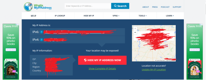
If you want to know your device’s IP address, go to this site-https://whatismyipaddress.com/. Here’s what the results were for my device’s IP address (and yes, I redacted my IP address information):
What can you deduce just from the information on this homepage? Let’s explain:
You can see both the IPv4 (IP version 4) and IPv6 (IP version 6) addresses for the device. Don’t worry, I’ll get into the differences between IPv4 and IPv6 later in this post.
You can also see the ISP (Internet Service Provider such as AT&T) along with the user’s current city, region and country. Even though the ISP field is a constant for the user, the user’s city, region, and country will reflect where the user is at the current moment, even if it’s not the user’s home city.
The map shows you where a user is currently located.
The two versions of IP addresses
As I mentioned above, your device will more often than not have both an IPv4 and an IPv6 address. However, you may be wondering what the differences are between these two types of IP addresses. Let’s dive in!
IP version 4
First off, let’s explore the world of IPv4 addresses. What exactly do they look like?
In this example, I’m showing the structure of IPv4 addresses using the most common IPv4 address-192.168.1.1 (which is a common default IP address for many home routers). Here are some things to know about the structure of IPv4 addresses:
IPv4 addresses are 32-bit/4-byte addresses, with each byte being represented by an octet (each of the 4 numbers represent one octet).
The reason each number in the IPv4 address is called an octet is because each number is stored as an 8-bit binary number.
Since each octet can be represented by a number from 0 to 255, there are roughly 4.2 billion possible combinations for IPv4 addresses (255^4).
IP version 6
Granted, 4.2 billion possible IP address combinations sounds like a lot, but given the amount of devices connected to the Internet these days, let’s just say we’ll need a lot more unique identifiers!
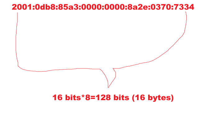
This is where IPv6 comes in. Let’s break down the structure of IPv6 addresses:
In this example, I’m showing the structure of IPv6 addresses, which is quite different from the structure of IPv4 addresses. Here’s a breakdown of the structure of IPv6 addresses:
Unlike IPv4 addresses, IPv6 addresses are stored in 8 sections of 16 bits apiece with each section being represented by a hexadecimal number.
In total, IPv6 addresses are 128 bits long.
Since each section of the IPv6 address can have up to 65,536 possible values, and there are 8 sections in an IPv6 address, there are 3.4*10^38 possible combinations for an IPv6 address. Just for context, that number is 340 undecillion (one with 66 zeroes)-this allows for a considerably larger range of IP addresses under IPv6 since IPv4 only allows for 4.2 billion possible IP addresses.
It’s subnetting time!
One more concept I want to discuss regarding IP addresses is subnetting. What are subnets in the world of IP addresses?
All IP addresses exist on a network on the wider Internet. However, these networks where IP addresses exist can be quite large. How can we make device-to-device communication more efficient on these networks?
Subnets (or subnet masks) help make device-to-device communication more manageable by splitting a network into two parts-a network ID and a host (or device) ID. Subnets are represented as 32-bit numbers that look like standard IPv4 addresses (e.g.: 255.255.255.0). The main benefit of subnets is that they allow devices to know which other devices are in their same network and which devices are in different networks and adjusts device-to-device communication accordingly.
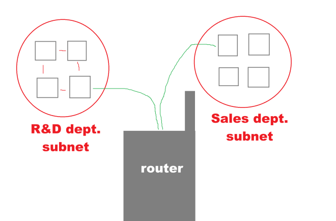
Let’s illustrate how subnets work:
Let’s say we’ve got two departments of a certain company-R&D (research and development) and sales and each department is part of the larger company’s Internet network. Let’s also assume that the R&D and the sales departments have their own distinct subnets. If one device on the R&D subnet wanted to send some information to another device on the R&D subnet, the first device would simply need to send a direct message to the second device. However, if a device on the R&D network wanted to send some information to a device on the Sales subnet, you’d be getting the handy-dandy router (or default gateway) to assist you in directing the information to the right network.
Now, how might subnetting work in the context of IP addresses? Let’s take the following two IP addresses-184.122.1.14 and 184.122.1.33 and let’s use the following subnet mask-255.255.255.0. Are these two IPs on the same subnet? Yes!
These two IPs are on the same subnet as the subnet (255.255.255.0) indicates that the first three octets of each IP must match, which they do!
CIDR, not CIDER
I did mention that subnets are written like standard IPv4 addresses (e.g.:255.255.255.0) but did you know there’s a convenient shorthand way to represent those subnets.
Introducing CIDR (not CIDER) notation, which stands for Classless Inter-Domain Routing Notation! The one thing you should know about CIDR notation is that it serves as an effective shorthand way of writing subnet masks.
How do you calculate a subnet mask in CIDR notation?
It’s actually pretty easy! Just convert each octet in the subnet into its binary form and count how many 1s appear. Since the subnet mask 255.255.255.0 has 24 ones in binary form, the subnet mask in CIDR notation can be represented as /24.
In other words, CIDR notation is represented as /[number of binary ones found in subnet].
Does IPv6 use subnets?
Yes and no. While IPv6 doesn’t use the same subnetting as IPv4, it does use something called prefixing, which works quite similar to subnetting in IPv4.
Both IPv4 and IPv6 use CIDR notation, but IPv6 tends to mostly work with the /64 mask as IPv6 addresses use the 64-bit-network/64-bit-host split.
Thank you for reading and following along on another great year of coding and tech! From C# to Tesseract readings to NBA predictions to IP addresses and even a little fun with HTML, I’ve certainly had fun with the content slate this year! Have a very merry and festive holiday season with your loved ones and see you in:
Yes dear readers, I’ve got so much awesome content to come in 2026 (including this blog’s 200th post)! Who knows what I’ll be covering-though you can bet on some juicy cybersecurity content headed your way!
Michael here, and in this post, I had one more Tesseract scenario I wanted to try-this one involving Tesseract translation and seeing how well Tesseract text in other languages can be translated to English. Let’s dive right in, shall we?
Let’s get stuff set up!
Before we dive into the juicy Tesseract translations, let’s first get our packages installed and modules imported on the IDE:
!pip install pytesseract
!pip install googletrans
import pytesseract
import numpy as np
from PIL import Image
from googletrans import Translator
Now, unlike our previous Tesseract scenarios, we’ll need to pip install an additional package this time-googletrans (pip install googletrans), which is an open-source library that connects to Google Translate’s API. Why is this package necessary? While Tesseract certainly has its capabilities when it comes to reading text from standard-font images (recall how Tesseract couldn’t quite grasp the text in OCR Scenario 2: How Well Can Tesseract Read Photos?, OCR Scenario 3: How Well Can Tesseract Read Documents? and OCR Scenario 4: How Well Can Tesseract Read My Handwriting?), one thing Tesseract cannot do is translate text from one language to another. Granted, it can read the text just fine, but googletrans will actually help us translate the text from one language to another. In this post, I’ll test the abilities of Tesseract in conjunction with googletrans to see not only how well Tesseract can read foreign language but also how well googletrans can translate the foreign text. I’ll test the Tesseract/googletrans conjunction with three different images in the following languages-Spanish, French, and German-and see how each image’s text is translated to English.
Leyendo el texto en Español (reading the Spanish text)
In our first Tesseract translation, we’ll attempt to read the text from and translate the following phrase from Spanish to English:
This phrase simply reads Tomorrow is Friday in English, but let’s see if our Tesseract/googletrans combination can pick up on the English translation.
First, we get the text that Tesseract read from the image:
As you can see, the googletrans Translator object worked its magic here with the translator method which takes three parameters-the text extracted from Tesseract, the text’s original language (Spanish or es) and the language that you want to use for text translation (English or en). The translated text is correct-the image’s text did read Tomorrow is friday in English. Personally, I’m amazed it managed to get the correct translation even though Tesseract didn’t pick up the enye (~) symbol when it read the text.
Now, you may be wondering why I added the await keyword in front of the translator.translate() method call-and here’s where I’ll introduce a new Python concept. See, the translator.translate() function is what’s known as an asynchronous function, which returns a coroutine object so that while the Google Translate API is being called and the translation is taking place, subsequent code in the program can be executed. Since the translator.translate() method is asynchronous, calling translation.text won’t return the translated text as the API request is still being made. Instead, this call will return an error, so to get around this, we’ll need to add the await keyword in front of translator.translate() before calling translator.text to be able to retrieve the translated text. The await keyword will make the program await the completion of the translation request from the Google Translate API before subsequent code is executed.
Granted the googletrans package did a good job of translating the text above from Spanish to English, but I want to see if the translator.translate() method can auto-detect the fact that the text is in Spanish and translate it to English:
In this example, I only specified that I want to translate the text to English without mentioning that the original text is in Spanish. Despite the small change, I still get the same desired translation-Tomorrow is friday.
I’ve noticed that when I use Google Translate, it can sometimes do a good job of auto-detecting the text’s language (though like any AI translation tool, it can also mis-detect the source language at times)
Traduisons ce texte français (Let’s translate this French text)
For my next scenario, we’re going to see how well the Tesseract/googletrans conjuction can translate the following French text:
Just as we did with the Spanish text image, let’s first read the text using Tesseract:
testImage = 'french text.png'
testImageNP = np.array(Image.open(testImage))
testImageTEXT = pytesseract.image_to_string(testImageNP)
print(testImageTEXT)

Joyeux
anniversaire a tol
OK, so a small misreading here (tol instead of the French pronoun toi), but pretty accurate otherwise. Perhaps Tesseract thought the lowercase i in toi was a lowercase l? Let’s see how this affects the French-to-English translation:
translator = Translator()
translation = await translator.translate(testImageTEXT, src='fr', dest='en')
print(translation.text)

Happy
birthday to you
Interestingly, even with the slight Tesseract misread of the French text, we still got the correct English translation of Happy birthday to you.
Deutsche Textübersetzung (German text translation)
Last but not least, we’ll see the Tesseract/googletrans conjuction’s capabilities on German-to-English text translation. Here’s the German text we’ll try to translate to English:
Now just as we did with the Spanish text and French text images, let’s first extract the German text from this image with Tesseract:
Let’s see what the resulting English translation is!
translator = Translator()
translation = await translator.translate(testImageTEXT, src='de', dest='en')
print(translation.text)

I love
Programming
really.
OK, so the actual phrase I put into Google translate was I really love programming and the German translation was Ich liebe Programmieren wirklich. Fair enough, right? However, the German-to-English translation of this phrase read I love programming really. How is this possible?
The translation quirk is possible because of the adverb in this case-wirklich (German for really). See, unlike English adverbs, German adverbs tend to be more flexible with where they’re placed in a sentence. So in English, “I love programming really” doesn’t sound too grammatically correct but in German, “Ich liebe Programmieren wirklich”-which places the adverb “really” after the thing it’s emphasizing “love programming”-is a more common way to use adverbs, as German adverbs tend to commonly be placed after the thing they’re emphasizing. And that is my linguistic fun fact for this post!
Towards the end of the previous post, we generated this equation to assist us in generating our linear regression NBA season predictions for this year. To recap what the equation means:
64.8 * (field goal %)
PLUS 113 * (3-point %)
PLUS 15.4 * (2-point %)
MINUS 1.94 * (seeding at end of season)
PLUS 0.011 * (total rebounds)
MINUS 0.00346 * (total assists)
PLUS 0.0215 * (total steals)
PLUS 0.00663 * (total blocks)
MINUS 0.0097 * (total turnovers)
MINUS 60.38 (the intercept)
That’s quite a mouthful, but I’ll show you the Python calculations we’ll be doing in order to generate those juicy predictions!
I’ll admit that even I’m not perfect with my blogs here, as I made a small mistake on the previous post that showed part of the equations as 215 * (total steals) rather than 0.0215 * (total steals). As it turns out, even experienced coders like me make oversights, so apologies for that!
A little disclaimer here
Before we dive in to our predictions, I want to clarify that these are simply win total/conference seeding predictions based off of a simple linear regression model configured by me. I personally wouldn’t use these predictions for any bets or parlays because first and foremost, I am your friendly neighborhood coding blogger, not your friendly neighborhood sportsbook. You can count on me for juicy, way-too-early predictions, but certainly not for any juicy over/unders.
If you do bet on NBA games this season, please do so responsibly! Thank you!
The way of the weighted averages
You may recall that for my post on last NBA season’s predictions, we used weighted averages to help generate the predictions. Since I personally liked that method, I’ll do so again.
Here’s the file with the weighted averages, which we’ll be using to calculate the predictions:
We’ll use the same methodology as we did last year for calculating the weighted averages, which went like this:
2022-23 to 2024-25 (last 3 seasons)-0.2 weight (higher weight for the three most recent seasons)
2019-20 to 2021-22 (three seasons prior to that)-0.1 (less weight for seasons further in the past, plus this timespan does include the two COVID shortened seasons)
2015-16 to 2018-19 (four seasons further back)-0.025 (even less weight for these seasons further in the past)
Now here’s the weighted averages file for all 30 teams:
Once I read the weighted averages CSV and ran the equation for all 30 teams, I get the predicted win totals for all 30 teams, which I will use for my way-too-early East/West seeding chart. Note that since the team names aren’t shown in the output, I took the liberty of manually adding each team name by each predicted win total so you know your favorite team’s projected win total (according to my model, of course).
One interesting difference between this year’s projected win totals and last year’s is the narrower range of possible win totals in this year’s model. See, the range of possible win totals in last year’s model was 24-54 wins, while the range of possible win totals in this year’s model is just 33-59 wins. Could the narrower possible win total range be due to the different features I used in this year’s model? It’ll be interesting to see how the season plays out.
Another interesting thing to note is that even though there is a narrower range of potential wins in this year’s model, the majority of teams’ win counts last season fell into this range-20 teams won between 33 and 59 games last season (Knicks, Pacers, Bucks, Pistons, Magic, Hawks, Bulls, Heat, Rockets, Lakers, Nuggets, Clippers, Timberwolves, Warriors, Grizzlies, Kings, Mavericks, Suns, TrailBlazers and Spurs).
How will the win counts look this time around? We’ll see as the season unfolds!
Michael’s Way-Too-Early Conference Seeding:
And now, for the stuff I really wanted to share with you all in this post: Michael’s Way-Too-Early Conference Seeding. Now that we’ve got our projected win totals for each team, it’s time to seed them in their projected spots! But that’s not all I’m going to do!
In addition to the model’s projected seedings, I’ll also give you my own personal seedings for all 30 teams. That’s right-this year, I want to see which set of predictions comes out more accurate-my predications or my model’s predictions. This will be fun to revisit next July once the season wraps up!
Eastern Conference predictions
To begin, let’s start with the model’s Eastern Conference predictions:
Play-Offs
Play-Ins
Maybe Next Year
1. Boston Celtics
7. Miami Heat
11. Toronto Raptors
2. Cleveland Cavaliers
8. Orlando Magic
12. Brooklyn Nets
3. Milwaukee Bucks
9. Chicago Bulls
13. Washington Wizards
4. New York Knicks
10. Atlanta Hawks
14. Charlotte Hornets
5. Indiana Pacers
15. Detroit Pistons
6. Philadelphia 76ers
And now, let’s see my personal Eastern Conference predictions:
Play-Offs
Play-Ins
Maybe Next Year
1. New York Knicks
7. Orlando Magic
11. Toronto Raptors
2. Cleveland Cavaliers
8. Milwaukee Bucks
12. Philadelphia 76ers
3. Boston Celtics
9. Atlanta Hawks
13. Brooklyn Nets
4. Detroit Pistons
10. Chicago Bulls
14. Charlotte Hornets
5. Miami Heat
15. Washington Wizards
6. Indiana Pacers
Here are some interesting observations about both the model’s predictions and my own personal predictions:
The Eastern Conference teams that made last season’s play-in (Heat, Hawks, Bulls, Magic) are the same ones projected to make another go at play-ins this year. In other words, could we see the same teams stuck in another year of play-ins?
Personally, I think the Hawks, Bulls and Magic will make another trip to the play-in. On the other hand, I think the Heat will eke out a 5 (maybe 6) seed in the East because of some great new acquisitions like small forward Simone Fontecchio and shooting guard Norman Powell.
I honestly don’t know why the model hates the Detroit Pistons, as it placed them at the bottom of the East once more. I ranked them as a possible 4-seed because after their improvement last year (44-38 from a dismal 14-68 in 2023-24), I feel they could be quite the playoff contender-and it was certainly nice to see 2021 1st Overall Pick Cade Cunningham finally develop into a star-quality player. The acquisition of the former Heat small forward Duncan Robinson should be exciting to see.
This might sound like a hot take here, but I don’t think the Sixers will even qualify for play-in, let alone playoffs given the plethora of issues they had last season. Least of all, Paul George and Joel Embiid-two of the biggest Sixers names-weren’t at the top of their game last season when they were healthy (and both of them missed significant time due to injuries).
Unlike my model, I think the Knicks could really take the top spot in the East this season. Despite falling just short of the 2025 NBA Finals, the Knicks showed they can certainly make a deep playoff run with talent such as Jalen Brunson (winner of the Clutch Player of the Year award), OG Anunoby and their acquisition of Karl-Anthony Towns from the Timberwolves during the 2024 offseason.
With two of the biggest names in the East-Jayson Tatum and Tyrese Haliburton-out for most if not all of this season due to Achilles injuries they got during last season’s playoffs, I think the East is wide open. Granted, I still think the Pacers and Celtics have a good chance at making the playoffs this year, but I don’t think either of them is a shoo-in for the top spot in the East, which in my opinion leaves the East playoff race wide open for another team to take the top spot (which as I said earlier, I think it could be the Knicks’ year to do just that). Also, I still think the Celtics could realistically clinch the 3-seed in the East despite the offseason departures of Jrue Holiday, Kristaps Porzingis, Al Horford and Luke Kornet, who were all key players in the Celtics 2024 Championship run.
Western Conference predictions:
First, let’s start with how the model think the Western Conference standings will play out this season:
Play-Offs
Play-Ins
Maybe Next Year
1. Oklahoma City Thunder
7. Golden State Warriors
11. Houston Rockets
2. LA Clippers
8. Phoenix Suns
12. Utah Jazz
3. Denver Nuggets
9. Sacramento Kings
13. New Orleans Pelicans
4. Memphis Grizzlies
10. Dallas Mavericks
14. Portland Trail Blazers
5. Minnesota Timberwolves
15. San Antonio Spurs
6. LA Lakers
Just as with the model’s Eastern Conference predictions, I certainly have disagreements with the Western Conference predictions. Here’s how I think the Western Conference standings will play out this season:
Play-Offs
Play-Ins
Maybe Next Year
1. Oklahoma City Thunder
7. Golden State Warriors
11. Dallas Mavericks
2. Houston Rockets
8. LA Clippers
12. Memphis Grizzlies
3. Minnesota Timberwolves
9. Sacramento Kings
13. Utah Jazz
4. Denver Nuggets
10. San Antonio Spurs
14. Portland Trail Blazers
5. Houston Rockets
15. New Orleans Pelicans
6. LA Lakers
As I did with my Eastern Conference predictions, here are some interesting observations between the model’s projected conference standings and my personal projected conference standings:
I’m sure the question on every NBA fan’s mind-including mine-is “Can the Oklahoma City Thunder pull off another championship?”. My guess-I think of all the champions we’ve seen in the 2020s alone, I think they’ve got the best shot at a repeat title. Why might that be? One big reason that could happen-the Thunder kept their core Big 3 (SGA, Chet Holmgren, and Jaylin Williams) around along with several other key players from the championship run such as Isaiah Hartenstein, Lu Dort, among others. Personally, I think that NBA teams would be wise not to go full rebuild-mode after winning their first championship, and it seems the Thunder have done just that (they only traded second-year small forward Dillon Jones, who played limited minutes in OKC’s championship run). Even if the Thunder don’t end up repeating as champions, I think, at the very least, the 1-seed in the West could be theirs for the taking once more.
Another interesting Western Conference storyline to watch would be whether Cooper Flagg (the 2025 #1 overall pick) becomes the next Luka Doncic for the Mavericks. After Doncic got traded for Anthony Davis during last year’s midseason trades, it’s safe to say the Mavericks’ season went south. A controversial trade and injuries to many key players-Anthony Davis (after the trade) and Kyrie Irving being the two most notable examples-didn’t help matters. Then again, having such an injury-struck roster to the point where the Mavericks nearly (but thankfully didn’t) have to forfeit games only added to their problems last season after the infamous Doncic-Davis trade. The drafting of 6’9″, 18-year-old forward Cooper Flagg could bring a spark to the struggling Mavericks (and from watching some of his highlights, I think Flagg has potential), but I think Flagg will need at least a year to gel with the Mavericks before they once again become Western Conference contenders.
Just as I was surprised that my model placed the Detroit Pistons at the bottom of the Eastern Conference given their improvements last season, I can say I’m just as surprised that the San Antonio Spurs were placed at the bottom of the Western Conference. Granted, they haven’t made the playoffs since 2019 and just went through a coaching change (Popovich stepped down and Mitch Johnson was named as head coach after serving as interim last season), but they did also improve their record from 22-60 in ’23-’24 to 34-48 last season. The Spurs also have their own solid Big 3 in De’Aaron Fox, Stephon Castle, and of course 2023 #1 overall pick Victor Wembanyama. Even though Wemby’s season was cut short last year due to deep vein thrombosis (a type of blood clot), his improved shooting and double-doubles could certainly help the Spurs once he’s fully recovered.
How might the Golden State Warriors do with their 35-and-over Big 3 (Jimmy Butler is 36, Draymond Green is 35, and Steph Curry is 37)? Given that they earned their playoff spot last season through play-ins, I’ve got a hunch that the Warriors might be seeing the play-ins once more-but will likely get a playoff spot in this manner. Yes, they had quite the herky-jerky trajectory last season, but the midseason acquisition of Jimmy Butler certainly gave them an extra spark down the regular season stretch-Butler’s basketball skills certainly paired well with guys like Steph and Draymond. Upsetting the 2-seeded Houston Rockets in the Western Conference quarterfinals last season certainly helps the Warriors’ momentum heading into this season, but I do wonder how the loss of their championship-winning forward Kevon Looney would affect the Warriors dynamic.
I know I said that I think the Thunder have a great chance to repeat as champions, but I also wonder if the Timberwolves would be a team to look out for in the 2026 postseason. After all, despite losing franchise mainstay Karl-Anthony Towns to the Knicks in the 2024 offseason, the Timberwolves adapted quite well as stars like Anthony Edwards and Naz Reid rose to the challenge by helping the team get to the Western Conference finals for the second year in a row (even though they got knocked out at the Western Conference finals for the second year in a row too). All in all, in terms of every NBA trade ever made, I think the Karl-Anthony towns trade-along with the players the Timberwolves got in exchange (Julius Randle and Donte DiVincenzo)-was one of the most even trades for both teams involved, as both the Knicks and Timberwolves made it to their respective conference finals.
Just as with my play-in predictions for the Eastern conference, at least three of the four projected play-in teams (according to the model) for the Western Conference made the play-ins last season-the Mavericks, Warriors, and Kings. I think the Warriors have the best shot at cracking the actual playoffs while the Mavericks could use another year for Cooper Flagg to develop (plus buy some time to get stars like Kyrie Irving back). It will be interesting to see how the Sacramento Kings fare because even though Domantis Sabonis, Zack LaVine and DeMar DeRozan fared well despite the disappointing finish, the talent around them could use some improvement. Perhaps the addition of Russell Westbrook (who’s in his 18th year in the NBA) could spice up the Kings’ offense, as he certainly showed he still had the athleticism and speed needed for basketball last season with the Denver Nuggets.
And now for something a little scandalous…
Boy oh boy this is certainly going to be the most interesting (or at least the most interestingly-timed) post I’ve written during this blog’s run. Why might that be?
Well, last Thursday (October 23, 2025) news broke that the FBI (US Federal Bureau of Investigation) had arrested 34 people for a pair of scandals that certainly rocked pro basketball-one involving colluding with Italian Mafia families (specifically the Gambino, Bonnano and Genovese crime families) to conduct a series of rigged poker games and another involved colluding to rig sports betting.
Here’s the wildest part though-among the 34 arrested were the current head coach of the Portland Trail Blazers (Chauncey Billups), a current Miami Heat star (Terry Rozier), and a former Cavaliers player (Damon Jones). Billups and Rozier were placed on leave by their respective teams.
Want to know some other juicy, scandalous details? Here are a few takeaways from the indictments:
Chauncey Billups was allegedly used by these Mafia families to lure in victims to the rigged poker games in order to make the poker games appear legitimate.
How the poker games were rigged is possibly the wildest part, with everything that was alleged to have happened sounding like it could’ve come from a James Bond movie. Among the methods used to rig these poker games were X-Ray tables that allowed these Mafia families to see opponents’ hands and rigged shuffling machines that could be used to predict what opponents’ hands would look like.
As for Rozier, the game that led to him being investigated was a March 23, 2023 game while Rozier was still with the Charlotte Hornets. In this game, Rozier left the game early due to a “foot injury”-which wasn’t true as Rozier conspired with a longtime friend of his that he planned to fake the “foot injury” in order to net this friend over $200,000 on his “under” statistics (that Rozier would underperform in the game in other words).
As for Damon Jones, he sold insider information to his co-conspirators during the 2022-23 season while working for the Lakers. The information concerned insider tips on lineup decisions and injury reports on star Lakers players; the co-conspirators were able to place significant wagers on their bets with this information. It was later revealed that one of the players whose injury report was leaked was LeBron James, who hasn’t been implicated in any wrongdoing.
All I will say is that it will be very very interesting to see not only how the rest of the NBA season plays out but also to see how commissioner Adam Silver will change league gambling policy-especially when it comes to players and coaching staff. Assuming other players and/or coaching staff get busted in the gambling ring (which could happen) the trials will be interesting-mostly because we’ll get to see who will snitch on who to get a sweet plea deal. Maybe there will be some RICO charges in the mix-which given what occurred, isn’t a stretch to think.
Anyway, thanks for reading as always, and enjoy the juicy action of the 2025-26 NBA season! The season is still young, so it’s anyone’s game!
All in all, after seeing how the season played out-I managed to get only 3/30 teams in the correct seeding. So what would I do here?
I’ll give my ML NBA machine learning predictions another go, also using data from the previous 10 seasons (2015-16 to 2024-25). You may be wondering why I’m trying to predict the outcomes of the upcoming NBA season once more given how off last year’s predictions were-the reason I’m giving the whole “Michael’s NBA crystal ball” thing another go is because I’m not only interested in how my predictions change from one season to the next but also because I plan to use a slightly different model than I did last year (it’ll still be good old linear regression, however) so I can analyze how different factors might play a role in a team’s record and ultimately their conference seeding.
So, without further ado, let’s jump right in to Michael’s Linear Regression NBA Season Predictions II!
Reading the data
Before we dive in to our juicy predictions, the first thing we need to do is read in the data to the IDE. Here’s the file:
Now let’s import the necessary packages and read in the data!
import pandas as pd
from sklearn.model_selection import train_test_split
from pandas.core.common import random_state
from sklearn.linear_model import LinearRegression
from google.colab import files
uploaded = files.upload()
import io

NBA = pd.read_excel(io.BytesIO(uploaded['NBA analysis 2025-26.xlsx']))
As you can see, we’ve still got all 31 features that we had in last year’s dataset-the only difference between this dataset and last year’s is the timeframe covered (this dataset starts with the 2015-16 and ends with the 2024-25 season).
Just like last year, this year’s edition of the predictions comes from http://basketball-reference.com, where you can search up plenty of juicy statistics from both the NBA and WNBA. Also, just like last year, the only thing I changed in the data from Basketball Reference is the Finish variable, which represents a team’s conference finish (seeding-wise) as opposed to divisional finish (since divisional finishes are largely irrelevant for a team’s playoff standings).
Now that we’ve read our file into the IDE, let’s create our model!
Creating the model
You may recall that last year, before we created the model, we used the Select-K-Best algorithm to help us pick the optimal model features. For a refresher, here’s what Select-K-Best chose for us:
['L', 'Finish', 'Age', 'FG%', '3P%']
After seeking the five best features for our model from the Select-K-Best algorithm, this is what we got. However, we’re not going to use the Select-K-Best suggestions this year as there are other factors I’d like to analyze when it comes to making upcoming season NBA predictions.
Granted, I’ll keep the Finish, FG%, and 3P% as I feel they provide some value to the model’s predictions, but I’ll also add a few more features of my own choosing:
X = NBA[['FG%', '3P%', '2P%', 'Finish', 'TRB', 'AST', 'STL', 'BLK', 'TOV']]
y = NBA['W']

X_train, X_test, y_train, y_test = train_test_split(X, y, test_size = 0.2, random_state = 0)
Along with the features I chose from last year’s model, I’ll also add the following other scoring categories:
2P%-The percentage of a team’s successful 2-pointers in a given season
TRB-A team’s total rebounds in a season
AST-A team’s total assists in a season
STL-A team’s total steals in a season
BLK-A team’s total blocks in a season
TOV-A team’s total turnovers in a season
The y-variable will still be W, as we’re still trying to predict an NBA team’s win total for the upcoming season based off of all our x-variables.
Now, let’s create a linear regression model object and run our predictions through that model object:
Just as with last year’s model, the predictions are run on the test dataset, which consists of the last 60 of the dataset’s 300 total records.
And now for the equation…
Now that we’ve generated predictions for our test dataset, let’s find out all of the coefficients and the intercept for the equation I will use to make this year’s NBA predictions:
Now that we know what our coefficients are, let’s see what this year’s equation looks like:
Although it’s much more of a mouthful than last year’s equation, it follows the same logic in that it uses the features of this year’s model in the order that I listed them:
A is FG%, B is 3P%, and so on until you get to I (which represents TOV).
Since all the coefficients are listed in scientific notation, I rounded them to two decimal places before converting them for this equation. Same thing for the intercept.
In case you’re wondering, no you can’t add all the coefficients together for this equation as each coefficient plays a part in the overall equation. Just like last year, we’re going to do the weighted-averages thing to generate projected win totals. Keep your eyes peeled for the next post, which covers the juicy predictions.
…and the accuracy test!
So now that we’ve got our 2025-26 NBA predictions model, let’s see how accurate it is:
from sklearn.metrics import mean_absolute_percentage_error

mean_absolute_percentage_error(y_test,yPredictions)

0.09573425883736708
Using the MASE (mean absolute percentage error) from sklearn like we did in last year’s analysis, we see that the model’s margin of error is roughly 9.57%. I’ll round that up to 10%, which means that despite not choosing the model’s features from a prebuilt algorithm, the overall accuracy of the model is still 90%.
Now, whether the model’s accuracy and my predictions hold up is something I’ll certainly revisit in 8 months time for another end-of-season reflection. After all, last season I only got 3 of the 30 teams in the correct seeding, though I did do better with predicting which teams didn’t make playoffs though.
Recall that to find the accuracy of the model using the MASE, subtract 100 from the (MASE * 100). Since the MASE rounds out to 10 as the nearest whole number (rounded to 2 decimal places), 100-10 gives us an accuracy of 90%
Last but not least, it’s prediction visualization time!
Before we go, the last thing I want to cover is how to visualize this year’s model’s predictions. Just like last year, we’re going to use the PYPLOT module from MATPLOTLIB:
import matplotlib.pyplot as plt

plt.scatter(y_test, yPredictions, color="red")
plt.xlabel('Actual values', size=15)
plt.ylabel('Predicted values', size=15)
plt.title('Actual vs Predicted values', size=15)
plt.show()
As you can see, the plot forms a sort of diagonal-line shape, which reinforces the model’s 90% prediction accuracy rate.
Also, just for comparison’s sake, here’s what my predictions looked like on last year’s model (the one where I used Select-K-Best to choose the model features):
This also looks like a diagonal-line shape, and last year’s model had a 91% accuracy rate.
Michael here, and in today’s post, we’ll take a look at how well Tesseract could possibly read a sample of my handwriting.
So far, we’ve tested Tesseract against standard computer-font text, a photo of a banner with text, and a common US tax document. Aside from the standard computer-font text, Tesseract didn’t work well with either the banner or the tax document.
However, can Tesseract work well with reading my handwriting? Let’s find out!
But first, a little pre-processing…
Before we test Tesseract on my handwriting, let’s follow the pre-processing steps we’ve followed for the other three Tesseract scenarios: pip install the necessary packages and import them onto the IDE.
Interestingly, Tesseract didn’t seem to pick up any text. I thought it might’ve picked up something, as the image simply contains black text on a white background. After all, there are no other objects in the image, nor is the information arranged like a document.
Could a little bit of image preprocessing be of any use with this image? Let’s find out!
Preprocessing time!
For this example, let’s try the same technique we used in the other two lessons-thresholding!
Next, let’s do a little thresholding on the image. Since the image is black font with white text, let’s see how a different thresholding technique (THRESH_BINARY_INV) might be able to assist us here:
The technique we used here-THRESH_BINARY_INV-is the opposite of what we used for the previous two lessons. In inverse binary thresholding, pixels above a certain threshold (127 in this case) turn black while pixels below this threshold turn white. I think this type of thresholding could be quite useful for handling black text on a white background, as was the case here.
Any luck reading?
Once we’ve done the thresholding, let’s see if that made a difference in the image’s Tesseract readability:
Interestingly, unlike the previous two Tesseract scenarios we tested (the photo of the banner and the W-2 document), no text was read at all after thresholding.
Honestly, I thought the handwriting scenario would do far better than the banner photo or W-2 given that the contents of this image are simply black text on a white background. I mean, Tesseract was able to perfectly read the image in The Seven-Year Coding Wonder, and that was red text on a lime-green background. I guess this goes to show that while Tesseract has its potential, it also has several limitations as we’ve discovered.
Michael here, and in today’s post, we’ll be testing out another OCR/Tesseract scenario-how well can Tesseract read documents?
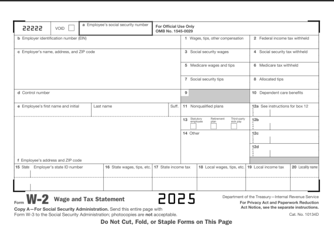
Here’s the document we’ll use for testing:
This is a standard-issue US W-2 form. For my international readers, a W-2 form is how US employees report their taxes to the federal government. All employee earnings and taxes withheld for a given calendar year are reported to the IRS (Internal Revenue Service, the agency that handles US taxpayer matters).
If you want to follow along with my Google Colab notebook, please save this image to your local drive and upload it to the IDE.
Let’s read the W-2
And now, let’s read in this W-2 form into our IDE. Before we start reading in the text to our IDE, let’s pip install the necessary packages if we don’t already have them:
OK, so using Tesseract, it appears we have some improvement from the previous scenario detailed in OCR Scenario 2: How Well Can Tesseract Read Photos? in the sense that text was even picked up at all. It appears that some sections of the W-2 form were even read perfectly (such as the line that read Do Not Cut, Fold, or Staple Forms on This Page). However, the bulk of the results appear to be complete gibberish, with a surprising amount of misread words (insimuctions instead of instructions, for example).
Now that we know how well Tesseract reads documents, let’s work some preprocessing magic to see if it yields any improvements in the text-reading process.
W-2 preprocessing
Could thresholding actually improve the Tesseract reading’s accuracy like it did for the photo test (granted, that was a marginal improvement, but it was still something).
Now that we’ve run the thresholding process on the image, let’s see how well it read the text:
w2TEXT = pytesseract.image_to_string(thresh)
print(w2TEXT)
vag
jen -urtbee EINE
" ¢ kirpleyo"s -ane. adeross. a
D Errplayers social
code
uray sunt
For Official Use Only
‘OMB No. 1545-0029
4 sans,
3. Seca seounty wae
5 Mo
7 Seca seounty 198,
andtps
|
B Allocaree s198
4 Corte naib 8 10. Lope~dent sare oe-otts
Te Eirpleyors frat “ar 1 Wa See natruct ons to Bax Te
° 13 125
14 Oe We
ta
f Eirployos's adaross ave £ * ence
18 Se EB Deiter 2 sraaes. ips. ote 18 Loca sages tps cto] 19 Lea noone tax
com WE=-2 wage and Tax Statement
Copy A—For Social Security Administration. Sere ths entire page
te the Social Securty Admin stratio7: onotoccpies are not acceptan e
born Ww.
cOes
Do Not Cut, Fold, or Staple Forms on This Page
ane
ot the
‘easy inter
For Privacy Act and Paperwork Reduction
‘Act Notice. see the separate instructions.
No.
349)
Granted, the original Tesseract reading of the W-2 form wasn’t that great, but wow this is considerably worse! I mean, what kind of a phrase is Errplayers social? However, I’ll give Tesseract some credit for surprisingly reading phrases such as the For Privacy Act and Paperwork Reduction correctly. Then again, I noticed the phrases in the document that Tesseract read the most accurately were the phrases in bold typeface.
Another one of Tesseract’s limitations?
Just as we saw when we tested Tesseract on the photo of the banner, we see that Tesseract has its limitations on reading documents as well. Interestingly enough, when we ran preprocessing on the photo of the banner, the preprocessing helped extract some text from the photo of the banner. However, when we ran the same preprocessing on the photo of the W-2, the reading came out worse than the reading we got from the original, un-processed image.
Why might that be? As you can see from the thresholding we did on the image of the W-2, most of the text in the form itself (namely the sections that contain people’s taxpayer information) comes out like it had been printed on a printer that was overdue for a black ink cartridge replacement. Thus, Tesseract wouldn’t have been able to properly read the text that came out of the image with the thresholding.
Then again, when Tesseract tried to read the text on the original, un-processed image, the results weren’t that great either. This could be because W-2 forms, like many legal forms, have a complex, multi-row layout that isn’t suited for Tesseract’s reading capabilities.
Personally, one reason I thought Tesseract would read this document better than the photo from the previous post is that the document’s text is not in a weird font and there’s nothing in the background of the document. I guess the results go to show that even with the things I just mentioned about the document, Tesseract still has its limitations.
Michael here, and in today’s post, we’ll see how well OCR and PyTesseract can read text from photos!
Here’s the photo we will be reading from:
This is a photo of a banner at Nashville Farmer’s Market, taken by me on August 29, 2025. I figured this would be a good example to testing how well OCR can read text from photos, as this banner contains elements in different colors, fonts, text sizes, and text alignments (I know you might not be able to notice at first glance, but the Nashville in the Nashville Farmers Market logo on the bottom right-hand corner of this banner is on a small yellow background).
Let’s begin!
But first, the setup!
Before we dive right in to text extraction, let’s read the image to the IDE and install & import any necessary packages. First, if you don’t already have these modules installed, run the following commands on either your IDE or CLI:
import pytesseract
import numpy as np
from PIL import Image
And now, let’s read the image!
Now that we’ve got all the necessary modules installed and imported, let’s read the image into the IDE:
testImage = 'farmers market sign.jpg'
testImageNP = np.array(Image.open(testImage))
testImageTEXT = pytesseract.image_to_string(testImageNP)
print(testImageTEXT)

Output: [no text read from image]
Unlike the 7 years image I used in the previous lesson, no text was picked up by PyTesseract from this image. Why could that be? I have a few theories as to why no text was read in this case:
There’s a lot going on in the background of the image (cars, pavilions, etc.)
PyTesseract might not be able to understand the fonts of any of the elements on the banner as they are not standard computer fonts
Some of the elements on the banner-specifically the Nashville Farmers’ Market logo on the bottom right hand corner of the banner don’t have horizontally-aligned text and/or the text is too small for PyTesseract to read.
Can we solve this issue? Let’s explore one possible method-image thresholding.
A little bit about thresholding
First of all, I figured we can try image thresholding to read the image text for two reasons: it might help PyTesseract read at least some of the banner text AND it’s a new concept I haven’t yet covered in this blog, so I figured I could teach you all something new in the process.
Now, as for image thresholding, it’s the process where grayscale images are converted to a two-colored image using a specific pixel threshold (more on that later). The two colors used in the new thresholding image are usually black and white; this helps emphasize the contrast between different elements in the image.
And now, let’s try some thresholding!
Now that we know a little bit about what image thresholding is, let’s try it on the banner image to see if we can extract at least some text from it.
First, let’s read the image into the IDE using cv2.read() and convert it to grayscale (thresholding only works with gray-scaled images):
The cv2.threshold() method takes four parameters-the grayscale image, the pixel threshold to apply to the image, the pixel value to use for conversion for pixels above and below the threshold, and the thresholding method to use-in this case, I’m using cv2.THRESH_BINARY.
Now, what is the significance of the numbers 127 and 255? 127 is the threshold value, which means that any pixel with an intensity less than or equal to this threshold will be set to black (intensity 0) while any pixel with an intensity above this value will be set to white (intensity 255). While 127 isn’t a required threshold value, it’s ideal because it’s like a midway point between the lowest and highest pixel intensity values (0 and 255, respectively). In other words, 127 is a quite useful threshold value for helping to establish black-and-white contrast in image thresholding. 255, on the other hand, represents the pixel intensity value to use for any pixels above the 127 intensity threshold. As I mentioned earlier, white pixels have an intensity of 255, so any pixels in the image above a 127 intensity are converted to a 255 intensity, so those pixels turns white while pixels at or below the threshold are converted to a 0 intensity (black).
A little bit about the ret parameter in the code: this value represent the pixel intensity threshold value you want to use for the image. Since we’re doing simple thresholding, ret can be used interchangeably with the thresholding value we specified here (127). For more advanced thresholding methods, ret will contain the calculated optimal threshold.
And now the big question…will Tesseract read any text with the new image?
Now that we’ve worked OpenCV’s thresholding magic onto the image, let’s see if PyTesseract picks up any text from the image:
bannerTEXT = pytesseract.image_to_string(thresh)
print(bannerTEXT)

a>
FU aba tee
RKET
Using the PyTesseract image_to_string() method on the new image, the only real improvement here is that there was even text read at all. It appears that even after thresholding the image, PyTesseract’s output didn’t even pick up anything close to what was on the banner (although it surprisingly did pick up the RKET from the logo on the banner).
All in all, this goes to show that even with some good image preprocessing methods, PyTesseract still has its limits. I still have several other scenarios that I will test with PyTesseract, so stay tuned for more!
Here’s the GitHub link to the Colab notebook used for this tutorial (you will need to upload the images again to the IDE, which can easily be done by copying the images from this post, saving them to your local drive, and re-uploading them to the notebook)-https://github.com/mfletcher2021/blogcode/blob/main/OCR_photo_text_extraction.ipynb.
Michael here, and today’s post will be a lesson on how to use bounding boxes in OCR.
You’ll recall that in my 7th anniversary post The Seven-Year Coding Wonder I did an introduction to Python OCR with the Tesseract package. Now, I’ll show you how to make bounding boxes, which you can use in your OCR analyses.
But first, what are bounding boxes?
That’s a very good question. Simply put, it’s a rectangular region that denotes the location of a specific object-be it text or something else-within a given space.
For instance, let’s take this restaurant sign. The rectangle I drew on the COME ON IN part of the sign would serve as a bounding box
In this case, the red rectangular bounding box would denote the location of the COME ON IN text.
You can use bounding boxes to find anything in an image, like other text, other icons on the sign, and even the shadow the sign casts on the sidewalk.
Bounding boxes, tesseract style!
Now that we’ve explained what bounding boxes are, it’s time to test them out on an image with Tesseract!
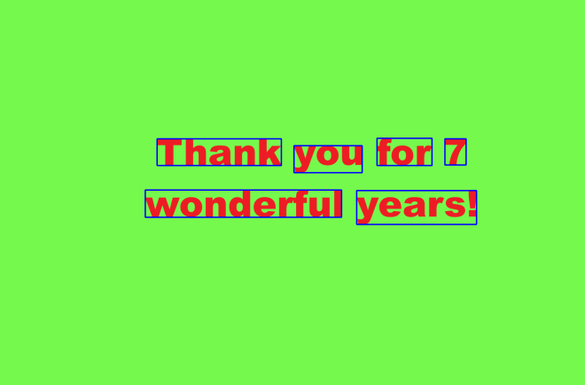
Here’s the image we’ll test our bounding boxes on:
Now, how do we get our bounding boxes? Here’s how:
Keep in mind, I will continue from where I left off on my 7-year anniversary post, so if you want to know how to read the image and print the text to the IDE, here’s the post you should read-The Seven-Year Coding Wonder.
First, install the OpenCV package:
!pip install opencv-python
Next, run pytesseract’s image_to_data() method on the image and print out the resulting dictionary:
Now, what does all of this juicy data mean? Let’s dissect it key-by-key:
level-The element level in Tesseract output (1 indicates page, 2 indicates block, 3 indicates paragraph, 4 indicates line and 5 indicates word)
page_num-The page number on the document where the object was found; granted, this is just a one-page image we’re working with, so this information isn’t terribly useful (though if we were working with a PDF or multi-page document, this would be very helpful information)
block_num-This indicates which chunk of connected text (paragraph, column, etc.) an element belongs to (this runs on a 0-index system, so 0 indicates the first chunk)
par_num-The paragraph number that a block element belongs to (also runs on a 0-index system)
line_num-The line number within a paragraph (also runs on a 0-index system)
word_num-The word number within a line (also runs on a 0-index system)
left & top-The X-coordinate for the left boundary and Y-coordinate for the top boundary of the bounding box, respectively
width & height-The width & height in pixels, respectively, of the bounding box
conf-The OCR confidence value (from 0-100, 100 being an exact match) that the correct word was detected in the bounding box. If you see a conf of -1, the element has no confidence value as its not a word
text-The actual text in the bounding box
Wow, that’s a lot of information to dissect! Another thing to note about the above output-not all of it is relevant. Let’s clean up the output to only display information related to the words in the image:
Granted, it’s not necessary to convert the image dictionary into a dataframe, but I chose to do so since dataframes are quite versatile and easy to filter. As you can see here, we have all the same metrics we got before, just for the words (which is what we really wanted).
And now, let’s see some bounding boxes!
Now that we know how to find all the information about an image’s bounding boxes, let’s figure out how to display them on the image. Granted, the pytesseract library won’t actually draw the boxes onto the images. However, we can use another familiar library to help us out here-OpenCV (which I did a series on in late 2023).
First, let’s install the opencv-python module onto our IDE if it’s not already there:
!pip install opencv-python
Remember, no need for the exclamation point at the front of the string if your running this command on a CLI.
After installing the opencv module in the IDE, we then read the image into the IDE using the cv2.imread() method. The cv2.IMREAD_COLOR ensures we read and display this image in its standard color format.
You may be wondering why we’re reading the image into the IDE again, especially after reading it in with pytersseract. We need to read the image again as pytesseract will only read the image string into the IDE, not the image itself. We need to read in the actual image in order to display the bounding boxes.
If you’re not using Google Colab as your IDE, no need to include this line-from google.colab.patches import cv2_imshow. The reason Google Colab makes you include this line is because the cv2.imshow() method caused Google Colab to crash, so think of this line as Google Colab’s fix to the problem. It’s annoying I know, but it’s just one of those IDE quirks.
Drawing the bounding boxes
Now that we’ve read the image into the IDE, it’s time for the best part-drawing the bounding boxes onto the image. Here’s how we can do that:
sevenYearsWords = sevenYearsWords.reset_index(drop=True)

howManyBoxes = len(sevenYearsWords['text'])

for h in range(howManyBoxes):
  (x, y, w, h) = (sevenYearsWords['left'][h], sevenYearsWords['top'][h], sevenYearsWords['width'][h], sevenYearsWords['height'][h])
  sevenYearsTestImage = cv2.rectangle(sevenYearsTestImage, (x, y), (x + w, y + h), (255, 0, 0), 3)

cv2_imshow(sevenYearsTestImage)
As you can see, we can now see our perfectly blue bounding boxes on each text element in this image. The process also worked like a charm, as each text element is captured perfectly inside each bounding box-then again, it helped that each text element had a 96 OCR confidence score (which ensured high detection accuracy).
How did we get these perfectly blue bounding boxes?
I first reset the index on the sevenYearsWords dataframe because when I first ran this code, I got an indexing error. Since the sevenYearsWords dataframe is essentially a subset of the larger sevenYearsDataFrame (the one with all elements, not just words), the indexing for the sevenYearsWords dataframe would be based off of the original dataframe, so I needed to use the reset_index() command to reset the indexes of the sevenYearsWords dataframe to start at 0.
Keep this method (reset_index()) in mind whenever you’re working with dataframes generated as subsets of larger dataframes.
howManyBoxes would let the IDE know how many bounding boxes need to be drawn-normally, you’d need as many bounding boxes as you have text elements
The loop is essentially iterating through the elements and drawing a bounding box on each one using the cv2.rectangle() method. The parameters for this method are: the image where you want to draw the bounding boxes, the x & y coordinates of each box, the x-coordinate plus width and y-coordinate plus height for each box, the BGR color tuple of the boxes, and the thickness of the boxes in pixels (I went with 3-px thick blue boxes).