Python Lesson 23: NumPy Copies & Views (NumPy pt. 6)

Advertisements

Hello everybody,

Michael here, and today’s lesson will be on using views and copies in NumPy arrays-this is part 6 in my NumPy series.

What exactly are copies and views in NumPy? Copies and views are both replications of a NumPy array, but with some major differences. A copy is a new array that’s created from a replication of another array while a view is simply a replication of an array rather than a new array entirely. A copy and the original array are stored in different locations in a computer’s memory while a view and the original array are stored in the same memory location.

Another major difference between NumPy copies and views is that copies own the original array’s data, thus, any changes made to a copy won’t affect the original array. On the other hands, views don’t own the original array’s data, thus, any changes made to a view will affect the original array.

Here’s an example of NumPy copies at work:

numpyA = np.array([12, 24, 36, 48, 60, 72])
A = numpyA.copy()
A[1] = 144

print(numpyA)
print(A)

[12 24 36 48 60 72]
[ 12 144  36  48  60  72]

And here’s an example of NumPy views at work:

numpyA = np.array([12, 24, 36, 48, 60, 72])
A = numpyA.view()
A[1] = 144

print(numpyA)
print(A)

[ 12 144  36  48  60  72]
[ 12 144  36  48  60  72]

In both examples, I modified the duplicate array (A in both examples) to replace the second element with 144. As you can see, in the copy example, 24 was replaced with 144 in the duplicate array but not in the original array. In the view example, 24 was replaced with 144 in both the duplicate array and original array.

Now, how can you find out if a replicated array is a copy or view? Take a look at this example:

numpyA = np.array([12, 24, 36, 48, 60, 72])

A = numpyA.view()
B = numpyA.copy()

print(A.base)
print(B.base)

[12 24 36 48 60 72]
None

To find out if an array is a copy or a view, use the .base attribute alongside the duplicated array. If the array is a copy, None will be returned. If the array is a view, the original array (numpyA in this example) will be returned.

Thanks for reading,

Michael

Python Lesson 21: Joining & Splitting NumPy Arrays (NumPy pt 4)

Advertisements

Hello everybody,

Michael here, and today’s lesson will be on joining and splitting NumPy arrays.

Joining NumPy arrays simply involves concatenating two or more NumPy arrays. However, joining two NumPy arrays isn’t as simple as joining two strings.

To join two or more NumPy arrays together, use the np.concatenate function. Here’s a simpleIn example of NumPy array concatenation:

numpy1 = np.array([0, 0.4, 0.8, 1.2, 1.6, 2])
numpy2 = np.array([2.4, 2.8, 3.2, 3.6, 4, 4.4])
numpy3 = np.concatenate((numpy1, numpy2))
print(numpy3)

[0.  0.4 0.8 1.2 1.6 2.  2.4 2.8 3.2 3.6 4.  4.4]

In order for the np.concatenate function to work properly, you’d need to pass in all the arrays you’d like to concatenate into a single tuple; if you pass in the arrays one-by-one, the function won’t work.

Also, when you concatenate multiple NumPy arrays, the dimensions stay the same:

print(numpy1.ndim)
print(numpy2.ndim)
print(numpy3.ndim)

1
1
1

Numpy1 and numpy2 are both 1-D arrays; the combined array numpy3 is also a 1-D array.

Now, can we join two arrays with different dimensions together? Let’s take a look:

numpy4 = np.array([[3, 6, 9], [4, 8, 12]])
numpy5 = np.array([5, 10, 15])
numpy6 = np.concatenate((numpy4, numpy5))
print(numpy6)

---------------------------------------------------------------------------
ValueError                                Traceback (most recent call last)
<ipython-input-14-479431df35d4> in <module>
      1 numpy4 = np.array([[3, 6, 9], [4, 8, 12]])
      2 numpy5 = np.array([5, 10, 15])
----> 3 numpy6 = np.concatenate((numpy4, numpy5))
      4 print(numpy6)

<__array_function__ internals> in concatenate(*args, **kwargs)

ValueError: all the input arrays must have same number of dimensions, but the array at index 0 has 2 dimension(s) and the array at index 1 has 1 dimension(s)

As you can see, trying to concatenate two arrays with different dimensions doesn’t work; all of the arrays you’re trying to concatenate must have the same number of dimensions.

Now, in the array concatenation examples I’ve shown you, the arrays are being joined along the same axis. How could you join arrays along different axes?

You would stack the arrays together. Here’s an example of NumPy array stacking:

numpy7 = np.array([14, 28, 42])
numpy8 = np.array([15, 30, 45])
numpy9 = np.stack((numpy7, numpy8), axis=1)
print(numpy9)

[[14 15]
 [28 30]
 [42 45]]

Stacking arrays is the same as concatenation, except stacking is usually done along a new axis. To stack a NumPy array, use the np.stack function and pass a tuple containing the arrays you want to stack and the axis you want to stack them on; if you don’t pass an axis into np.stack, arrays will automatically be stacked along the first axis.

What would it look like if these arrays were stacked along the first axis rather than the second axis? Take a look:

numpy7 = np.array([14, 28, 42])
numpy8 = np.array([15, 30, 45])
numpy9 = np.stack((numpy7, numpy8))
print(numpy9)

[[14 28 42]
 [15 30 45]]

All of the elements from both arrays will still be present, however, stacking along the first axis creates a 2×3 array, while stacking along the second axis creates a 3×2 array. Both stacked arrays are still 2-D.

  • In case you didn’t figure it out, axis=0 refers to the first axis while axis=1 refers to the second axis.
  • You can’t stack along a non-existent axis; in this example, the stacked array only has two dimensions, therefore you can’t stack along axis=2 because the stacked array has no third dimension and thus has no third axis.

Stacking along axes works well, but what are some other NumPy array stacking methods?

Let’s say you wanted to stack along rows. Here’s how to do so:

numpy7 = np.array([14, 28, 42])
numpy8 = np.array([15, 30, 45])
numpy9 = np.hstack((numpy7, numpy8))
print(numpy9)

[14 28 42 15 30 45]

To stack an array along rows, use the np.hstack function and pass in a tuple containing the arrays you want to stack. In this example, stacking along rows simply merged the two arrays into a single 1-D array with the elements of numpy7 being listed before numpy8.

Now what if you wanted to stack along columns? Here’s how to do so:

numpy7 = np.array([14, 28, 42])
numpy8 = np.array([15, 30, 45])
numpy9 = np.vstack((numpy7, numpy8))
print(numpy9)

[[14 28 42]
 [15 30 45]]

To stack arrays along columns, use the np.vstack function-the parameter for this function is the same as the parameter for the np.hstack function (a tuple containing the arrays you want to stack). In the example, stacking along columns created a 2×3 2-D array (this is the same outcome as stacking along the first axis).

Now, there’s another way that you can stack your array-along depth (or height). Here’s how to do so:

numpy7 = np.array([14, 28, 42])
numpy8 = np.array([15, 30, 45])
numpy9 = np.dstack((numpy7, numpy8))
print(numpy9)

[[[14 15]
  [28 30]
  [42 45]]]

Stacking along depth/height is the same gist as stacking along rows or columns-the only difference is that you’d use the np.dstack function to stack along depth/height. In this example, stacking along depth/height created a 3×2 3-D array, which is interesting because in the example where I stacked along the 2nd axis in a previous example (using the same three NumPy arrays), I got a 3×2 2-D array.

Now that we’ve discussed the basics of joining NumPy arrays, let’s discover how to do the reverse (splitting arrays).

Here’s a simple example of splitting a NumPy array:

numpy10 = np.array([100, 200, 300, 400, 500, 600, 700, 800, 900, 1000])
numpy11 = np.array_split(numpy10, 2)
print(numpy11)

[array([100, 200, 300, 400, 500]), array([ 600,  700,  800,  900, 1000])]

To split up a NumPy array, use the np.array_split function and pass in two parameters-the array you want to split up and the number of splits you want to use on the array. In this example, I have an array of 10 elements that I split in two.

Something to note when splitting areas is that the number of splits you want to use on an array doesn’t need to be divisible by the number of elements in the array. Granted, I did use two splits on a 10-element array. Watch what happens when I use three splits on the same 10-element array:

numpy10 = np.array([100, 200, 300, 400, 500, 600, 700, 800, 900, 1000])
numpy11 = np.array_split(numpy10, 3)
print(numpy11)

[array([100, 200, 300, 400]), array([500, 600, 700]), array([ 800,  900, 1000])]

The split still works, though the array isn’t split evenly (and Python automatically decides how to split the array).

Now let’s say you wanted to access one of the individual arrays. Here’s how to do so (using the 3-split example):

print(numpy11[0])
print(numpy11[1])
print(numpy11[2])

[100 200 300 400]
[500 600 700]
[ 800  900 1000]

Accessing individual arrays from a larger split NumPy array is the same as accessing elements from an individual array-in this case, the first array is index 0, the second array is index 1, and so on.

Now what if we wanted to access individual elements from these split arrays? Take a look at this example:

print(numpy11[0][1])
print(numpy11[1][1])
print(numpy11[2][1])

200
600
900

To access an individual element in each individual array, you’d need to add another indexing call. In this example, the first indexing call refers to the array itself while the second indexing call refers to the element inside the array.

Now, how would you split a multi-dimensional array? Take a look at this example:

numpy12 = np.array([[200, 400, 600, 800, 1000, 1200], [300, 600, 900, 1200, 1500, 1800]])
numpy13 = np.array_split(numpy12, 2)
print(numpy13)

[array([[ 200,  400,  600,  800, 1000, 1200]]), array([[ 300,  600,  900, 1200, 1500, 1800]])]

In this example, I am splitting a 2-D array in two-interestingly enough, both of the split arrays are still 2-D.

As you can see in the example, there are two 1-D arrays inside the 2-D array, therefore, splitting the 2-D array in two made sense. However, what if you wanted to split this 2-D array another way? Let’s see what happens when we split this array in three:

numpy12 = np.array([[200, 400, 600, 800, 1000, 1200], [300, 600, 900, 1200, 1500, 1800]])
numpy13 = np.array_split(numpy12, 3)
print(numpy13)

[array([[ 200,  400,  600,  800, 1000, 1200]]), array([[ 300,  600,  900, 1200, 1500, 1800]]), array([], shape=(0, 6), dtype=int32)]

When you split this array in three, you get both of the 1-D arrays in the 2-D arrays plus a blank array with a shape of (0, 6). If I was to split this array in four, I would’ve gotten both of the 1-D arrays plus two blank arrays with a shape of (0, 6).

A neat thing about splitting arrays is that, just like with joining arrays, you can split the arrays along a certain axis. Let’s see how axis-splitting an array works with a 2-D array:

numpy14 = np.array([[22, 44, 66, 88, 110], [33, 66, 99, 132, 165]])
numpy15 = np.array_split(numpy14, 5, axis=1)
print(numpy15)

[array([[22],
       [33]]), array([[44],
       [66]]), array([[66],
       [99]]), array([[ 88],
       [132]]), array([[110],
       [165]])]

In this example, I split the 2-D array numpy14 in five, resulting in a split array where elements from both of the 1-D arrays are stacked on top of each other in two columns. To split a NumPy array along a certain axis, specify the axis you want to split along after the number of splits you want to perform.

  • Just as with axis-joining an array, if you don’t specify an axis to split along in the np.array_split function, the array will automatically split along the first axis.
  • You can’t split along an axis beyond the scope of the array. In this example, since numpy14 is a 2-D array, you can’t split along axis=2 since a 2-D array doesn’t have a third axis.

Now, I mentioned that you can join arrays along rows, columns, and depth/height. However, did you know that each of the array-joining functions-np.hstack, np.vstack, and np.dstack-also have array-splitting counterparts-np.hsplit, np.vsplit, np.dsplit?

Let’s demonstrate the np.hsplit function first, which splits your array along rows:

numpy16 = np.array([40, 80, 120, 160, 200, 240])
numpy17 = np.hsplit(numpy16, 2)
print(numpy17)

[array([ 40,  80, 120]), array([160, 200, 240])]

In this example, I split numpy16 in two along rows; as you can see, both split arrays are displayed along a single row. Also, even though np.hsplit is the counterpart to np.hstack, np.hsplit doesn’t require a tuple as a parameter since you’re splitting a single array rather than stacking multiple arrays on top of each other.

Now let’s check out the np.vsplit function, which splits your array along columns:

numpy18 = np.array([[2010, 2011, 2012, 2013], [2014, 2015, 2016, 2017], [2018, 2019, 2020, 2021]])
numpy19 = np.vsplit(numpy18, 3)
print(numpy19)

[array([[2010, 2011, 2012, 2013]]), array([[2014, 2015, 2016, 2017]]), array([[2018, 2019, 2020, 2021]])]

Interestingly, the output for np.vsplit is displayed in the same format as the output for np.hsplit. However, keep in mind that unlike for np.hsplit, np.vsplit won’t work on 1-D arrays-you’ll need at least a 2-D array to make np.vsplit work.

Finally, let’s demonstrate the np.dsplit function, which splits your array along depth/height:

numpy20 = np.array([[[1996, 1997, 1998, 1999], [2000, 2001, 2002, 2003], [2004, 2005, 2006, 2007]]])
numpy21 = np.dsplit(numpy20, 4)
print(numpy21)

[array([[[1996],
        [2000],
        [2004]]]), array([[[1997],
        [2001],
        [2005]]]), array([[[1998],
        [2002],
        [2006]]]), array([[[1999],
        [2003],
        [2007]]])]

Unlike the output for np.hsplit and np.vsplit, the output for np.dsplit displays stacked, with elements from each 1-D array interspersed with each other. Also, for np.dsplit to work, you’ll need at least a 3-D array; 2-D arrays won’t work with np.dsplit.

Thanks for reading,

Michael

Python Lesson 20: Indexing, Slicing, and Iterating Through NumPy Arrays (NumPy pt. 3)

Advertisements

Hello everybody,

Michael here, and today’s lesson will be on indexing, slicing, and iterating through NumPy arrays-this is part 3 in my NumPy series.

First off, let’s discuss how to access elements in NumPy arrays. Here’s a simple example of this:

arrA = np.array([7, 14, 21, 28, 35, 42])
print(arrA[2])

21

As you can see, accessing elements in NumPy arrays is similar to accessing elements in regular Python arrays.

But that was just a simple 1-D array. How would you access elements from a 2-D array?

arrB = np.array([[9, 18, 27, 36, 45], [11, 22, 33, 44, 55]])
print(arrB[0, 2])

27

Turns out, accessing elements from a 2-D array is simple as well, except you’d use two parameters rather than just one. The first parameter specifies which dimension you’d like to search in and the second parameter specifies the element in that dimension you’d like to retrieve. In this example, I’m retrieving the third element from the first dimension (recall that Python arrays have an indexing system that starts with 0).

Simple enough right? Now let’s see how we can access elements from a 3-D array:

arrC = np.array([[[12, 24, 36, 48, 60], [13, 26, 39, 52, 65], [14, 28, 42, 56, 70]], [[20, 40, 60, 80, 100], [21, 42, 63, 84, 105], [22, 44, 66, 88, 110]]])
print(arrC[1, 2, 1])

44

This one is a bit more complex since there is more to break down, but there’s an easy way to explain 3-D array indexing. First of all, since there are three dimensions, there are obviously three parameters you’d need to use.

Aside from that, the first parameter is 1, which tells Python to look for an element in the second dimension. The second parameter is 2, which narrows the search down to the third array within the second dimension. The third parameter is 1, which further narrows down the search to the second element within the third array within the second dimension-the element that is returned from this search is 44.

Now let’s demonstrate how to perform negative (or reverse) indexing on a 1-D array:

arrD = np.array([0.2, 0.4, 0.6, 0.8, 1, 1.2, 1.4])
print(arrD[-2])

1.2

Reverse indexing on a NumPy array is the same as reverse indexing on a regular Python array. In this example, I am retrieving the element at index -2 (1.2), which refers to the second index from the right of the array.

Now here’s reverse indexing at work on a multi-dimensional array:

arrE = np.array([[-12, -9, -6, -3, 0], [-28, -21, -14, -7, 0], [-32, -24, -16, -8, -0]])
print(arrE[1, -1])

0

Reverse indexing on a multi-dimensional array is also fairly simple. In this example, I am retrieving the last element (or rightmost element) from the second array-within-an-array.

One more neat thing about NumPy array indexing is that it allows you to perform basic arithmetic on certain elements of the array. Here’s an example of that:

arrF = np.array([2, 4, 8, 16, 32, 64, 128, 256, 512, 1024, 2048])
print(arrF[2]+arrF[-2])
print(arrF[3]-arrF[0])
print(arrF[-1]*arrF[1])
print(arrF[2]/arrF[0])
print(arrF[2]**2)

1032
14
8192
4.0
64

In this example, I am performing the four basic arithmetic operations (addition, multiplication, subtraction, and division) and exponentiation (raising a number to a certain power) on certain elements in the array; I’m using different elements for each operation.

Next up, let’s discuss slicing an array. In the context of programming, array slicing is when you take certain element(s)/portion(s) from an array to create a new, smaller array. Here’s a simple example of NumPy array slicing:

arrG = np.array([1982, 1986, 1990, 1994, 1998, 2002, 2006, 2010, 2014, 2018, 2022])
print(arrG[0:5])

[1982 1986 1990 1994 1998]

In this example, Python is printing out the first five elements of arrG. Recall that when retrieving a range of elements from an array, the element corresponding to the end index is not included-so in this case, the 6th element wasn’t included.

Now, just as with regular Python arrays, you can slice arrays without a start index or end index-you just need one of these indexes to slice an array. Let me show you what I’m talking about:

print(arrG[5:])

[2002 2006 2010 2014 2018 2022]

In this example, I used [5:] to retrieve the sixth element in the array onward.

print(arrG[:5])

[1982 1986 1990 1994 1998]

In this example, I used [:5] to retrieve all elements in the array up to BUT NOT INCLUDING the sixth element.

The next topic I want to discuss is negative (or reverse) slicing; just as you can perform reverse indexing on an array, you can also perform reverse slicing on an array as well.

Let me show you an example of reverse slicing:

print(arrG[-4:-1])

[2010 2014 2018]

Reverse slicing has the same idea as reverse indexing-indexing starts at -1, which corresponds to the rightmost element in the array (2022 in the case of arrG).

If I wanted to include 2022 in my reverse slicing, I would’ve used this code:

print(arrG[-4:])

[2010 2014 2018 2022]

Had I used the line print(arrG[-4:0]), I would’ve recieved an empty array as output.

Now let’s explore a new array concept that I haven’t discussed here before-the concept of step. The step concept allows you to set a step for the slicing (e.g. return every other element, etc.).

Let’s see a simple example of slicing an array by step:

print(arrG[::3])

[1982 1994 2006 2018]

In this example, I retrieved every third element from arrG starting with the first element-1982. In other words, I retrieved the 1st, 4th, 7th, and 10th elements from arrG.

Now what if I wanted to perform step slicing only on a certain portion of the array:

print(arrG[0:6:2])

[1982 1990 1998]

In this example, I am performing step slicing on the 1st-7th elements of arrG (which correspond to indexes 0-6) by retrieving every other element from this portion of the array. If you want to perform step slicing on a portion of the array (rather than the whole array), you need to specify the portion of the array you would like to slice in the first two parameters-in this example, since I wanted to perform my slicing on elements 1-7, I used 0 and 6 as the first two parameters in the above example.

Now, how would we slice multi-dimensional arrays? Here’s an example (using a 2-D array):

arrH = np.array([[22, 44, 66, 88, 100], [33, 66, 99, 132, 165]])
print(arrH[0, 1:4])

[44 66 88]

In this example, the slicing function (referring to the line arrH[0, 1:4]) has two parameters rather than one-the first parameter contains the dimension where you wish to perform the slicing and the second parameter contains the range of elements you would like to retrieve (up to but not including the end index).

In the slicing function, I retrieved the 2nd through 4th elements (indexes 1-4) in the first dimension of the array (index 0). Step slicing also works for multi-dimensional arrays; for instance, the line print(arrH[0, ::2]) would have worked here (and it would have returned the 1st, 3rd, and 5th elements from the 1st dimension).

Now, how would we go about slicing a 3-D array? Take a look at the example below:

arrI = np.array([[[0, -9, -18, -27, -36], [0, -8, -16, -24, -32], [0, -7, -14, -21, -28]]])
print(arrI[0, 1, 0:3])

[  0  -8 -16]

In order to slice a 3-D array, you’d need 3 parameters for the slicing function-the first parameter represents the 2-D array within the 3-D array where you wish to perform the slicing, the second parameter represents narrows the slicing focus to a 1-D array within the 2-D array you selected, and the third parameter represents the range of elements in the 1-D array that you want to retrieve.

In this example, the first parameter is 0, which tells Python to start the array slicing in the first (and only) 2-D array within the 3-D array. The next parameter is 1, which tells Python to narrow the array slicing focus to the second 1-D array within the 2-D array. The last parameter is 0:3, which tells Python to retrieve the 1st-3rd elements from the second 1-D array within the 2-D array.

Last but not least, let’s explore how to iterate through NumPy arrays (which involves looping through all array elements).

To iterate through NumPy arrays, a for loop while do the trick. Here’s an example of iterating through a 1-D array:

arrJ = np.arange(10, 75, 5, int)
print(arrJ)

[10 15 20 25 30 35 40 45 50 55 60 65 70]
for x in arrJ:
    print(x)

10
15
20
25
30
35
40
45
50
55
60
65
70

To iterate through a simple 1-D array, all you need is the lines for x in [array name]: print(x). Not hard at all.

Let me discuss the arange function I used. The arange function is simply another way to create a NumPy array; this function has 4 parameters-the first element in the array, the last element in the array, the increment/decrement that is used to generate each element of the array, and the number type of the elements in the array (you usually use int or float).

Now let’s demonstrate iterating through a 2-D array:

arrK = np.array([[1, 1, 2, 3, 5, 8], [13, 21, 34, 55, 89, 144]])

for y in arrK:
    print(y)

[1, 1, 2, 3, 5, 8]
[13, 21, 34, 55, 89, 144]

Looks good right? The for loop syntax I used might work if you want to iterate through each 1-D array but this doesn’t work if you want to iterate through each element (known in programming lingo as a scalar) in each array-within-an-array.

Here’s how to iterate through each 1-D array in the 2-D array:

for x in arrK:
    for y in x:
        print(y)

1
1
2
3
5
8
13
21
34
55
89
144

A simple way to iterate through multi-dimensional arrays is the use of nested for loops. In this example, the outer for loop iterates through the main 2-D array while the inner for loop iterates through each element in each 1-D array within the 2-D array.

This is a great way to iterate through multi-dimensional arrays, but here’s an even better way to iterate through multi-dimensional arrays:

for x in np.nditer(arrK):
    print(x)

1
1
2
3
5
8
13
21
34
55
89
144

Simply using NumPy’s nditer function (and passing your array as a parameter) will iterate through each element in your array with just a simple line of code. The nditer function is super helpful because it allows you to iterate through a multi-dimensional array with a single line of code; recall that NumPy arrays can go up to 32-D, which would make for a very cumbersome-to-write nested for loop.

Now check out the two methods when used for iterating through a 3-D array. Which do you think is more efficient?

arrL = np.array([[[2, 4, 8, 16, 32], [3, 9, 27, 81, 243], [4, 16, 64, 256, 1024]]])

for x in arrL:
    for y in x:
        for z in y:
            print(z)

2
4
8
16
32
3
9
27
81
243
4
16
64
256
1024
for x in np.nditer(arrL):
    print(x)

2
4
8
16
32
3
9
27
81
243
4
16
64
256
1024

As you can see, both methods work great for iterating through arrL. However, the nditer method is more efficient and accomplishes the iterating with one line of code (the nested for loops method uses three lines of code).

Finally, I wanted to discuss step iterating through an array. Just as you can perform step slicing on an array, you can also step iterate through an array too:

for x in np.nditer(arrL[:, ::3]):
    print(x)

2
4
8
16
32

In this example, I am iterating through arrL but only returning every third element.

  • For step slicing and step iteration, remember that the step starts with the first element in the array unless you specify otherwise!

Thanks for reading,

Michael

Python Lesson 19: NumPy Array Shaping (NumPy pt.2)

Advertisements

Hello everybody,

Michael here, and today’s post will on how to manipulate the shape of arrays in NumPy-this is the second lesson in my NumPy series.

Now, before we get started, let’s remember to import NumPy to our IDE using the line import numpy as np.

  • Remember to pip install numpy if you haven’t done so already! Also, if you’re not sure if you’ve already got NumPy, use the pip list command to check.

Now that the import has been taken care of, let’s first demonstrate how to find the shape of a NumPy array:

arrayA = np.array([[0.5, 1, 1.5, 2, 2.5, 3], [3.5, 4, 4.5, 5, 5.5, 6]])
print(arrayA.shape)

(2, 6)

In this example, I created a 2-D array with six elements in each array. To find out the array’s shape, I called the array’s .shape function. The shape is shown as (2, 6), which means that this array has 2 dimensions and 6 elements per dimension.

Now how would we reshape this array? Let’s say that we wanted to turn this 2-D array into a 3-D array. Here’s how we would do that:

arrayB = arrayA.reshape(3, 4)
print(arrayB.shape)
print(arrayB)

(3, 4)
[[0.5 1.  1.5 2. ]
 [2.5 3.  3.5 4. ]
 [4.5 5.  5.5 6. ]]

To reshape a NumPy array, use the .reshape function on your current array and change the parameters of the .reshape function to the dimensions you want the new array to have.

In this example, I changed the shape of arrayA to 3 X 4, which means that the new array (stored in the arrayB variable) will have 3 dimensions with 4 elements in each dimension.

Look, the .reshape function is quite versatile, but you can just use any two numbers as the parameters here. Here’s what happened when I tried reshaping arrayA to 5×7:

arrayC = arrayA.reshape(5, 7)
print(arrayC)

---------------------------------------------------------------------------
ValueError                                Traceback (most recent call last)
<ipython-input-6-70ed58b6935b> in <module>
----> 1 arrayC = arrayA.reshape(5, 7)
      2 print(arrayC)

ValueError: cannot reshape array of size 12 into shape (5,7)

Since 5 and 7 aren’t factors of 12 (the array size), Python couldn’t reshape the array to 5×7.

In order to know all of the possible ways that you can shape the array, count all of the elements in the array (12 in the case of arrayA) then make a note of all of the factors of that amount. Since there are 12 elements in arrayA, the possible shapes arrayA can take include (1, 12), (2, 6), and (3, 4), as these are all number pairs that have a product of 12.

  • (12, 1), (6, 2), and (4, 3) work as well-recall that, from the Commutative Property of Multiplication, you can switch the order of the factors around and get the same product. However, keep in mind that the dimensions will be different if you switch the order of the numbers.
  • Also, when reshaping the array, keep in mind that dimensions are capped at size 32 (I mentioned this in the previous lesson)

Now I’ve demonstrated how to reshape a NumPy array with a standard number-pair tuple. However, did you know that you can also include an unknown dimension. Here’s how that works:

arrayD = np.array([0, 3, 6, 9, 12, 15, 18, 21, 24, 27])

arrayE = arrayD.reshape(2, -1)
print(arrayE)

[[ 0  3  6  9 12]
 [15 18 21 24 27]]

Yes, NumPy allows you to use -1 as a shape parameter in the .reshape method. But what does this mean? -1 simply represents an unknown dimension that you want NumPy to figure out. How does NumPy figure out this unknown dimension? It looks at the length of the array and the known dimension(s) in order to determine how to best shape the array. In this example, NumPy sees that the known dimension is 2, so the array is shaped to have two rows with five elements per row-the array has 10 elements, so 10 divided by 2 (# of rows) equals 5 (# of elements per row).

Now what if I had switched the order of the parameters in the .reshape function to (-1, 2). What would we get?

arrayF = arrayD.reshape(-1, 2)
print(arrayF)

[[ 0  3]
 [ 6  9]
 [12 15]
 [18 21]
 [24 27]]

If I switch the order of the .reshape function parameters to (-1, 2), the array would still have 10 elements but instead of 2 rows-by-5 columns, I get an array with 5 rows-by-2 columns.

As you can see, using the unknown dimension trick of -1 works just great with two shape parameters. However, the -1 trick also works with three shape parameters. Take a look at the example below:

arrayG = arrayD.reshape(2, 5, -1)
print(arrayG)

[[[ 0]
  [ 3]
  [ 6]
  [ 9]
  [12]]

 [[15]
  [18]
  [21]
  [24]
  [27]]]

In this example, using -1 as a third shape parameter splits the array into two 5×1 arrays.

Now what if I still used three shape parameters, but placed the -1 as the second shape parameter?

arrayH = arrayD.reshape(2, -1, 5)
print(arrayH)

[[[ 0  3  6  9 12]]

 [[15 18 21 24 27]]]

In this example, using -1 as the second shape parameter still splits the array in two, except you get two 1×5 arrays.

  • You can only have one unknown dimension in every .reshape function!
  • For all of the known dimensions, you can only include factors of the array length. In other words, since arrayD has a length of 10, you could only use 1, 2, 5, or 10 for the known dimension(s), as these are all the factors of 10.

The next NumPy trick I will show you is how to flatten arrays. In NumPy, you can convert multi-dimensional arrays into 1-D arrays-this is called flattening the array-with a simple line of code. Here’s how to flatten a NumPy array:

arrayI = np.array([[4, 8, 12], [5, 10, 15], [6, 12, 18]])
arrayJ = arrayI.reshape(-1)
print(arrayJ)

[ 4  8 12  5 10 15  6 12 18]

To flatten a NumPy array, simply use the .reshape function with the -1 parameter. That’s it. However, for the flattening to work, only use the -1 shape parameter-don’t include other shape parameters!

Now I know I said that the array-flattening trick works with multi-dimensional arrays, but it also works with 0-D arrays. Here’s an example of this:

arrayK = np.array(7)
arrayL = arrayK.reshape(-1)
print(arrayL)

[7]

As you can see, my 0-D was successfully turned into a 1-D array.

Last but not least, I want to show you two special NumPy functions that you will likely encounter if you’re learning about more advanced Python topics (e.g. computer vision)-.zeros and .ones. These functions allow you to create arrays of zeros and ones, respectively (recall that 0 and 1 are the two elements in the binary number system from Java Lesson 5: Java Numbering Systems).

First, let’s create an array of zeros:

arrayM = np.zeros((4,4), int)
print(arrayM)

[[0 0 0 0]
 [0 0 0 0]
 [0 0 0 0]
 [0 0 0 0]]

In this .zeros function, I used two parameters-a tuple to specify the shape of the array (4×4) and a value to specify the type to store the zeros (int).

Let’s say I didn’t specify a value type for the zeros. How would they be stored on the program?

arrayM = np.zeros((4,4))
print(arrayM)
print(arrayM.dtype)

[[0. 0. 0. 0.]
 [0. 0. 0. 0.]
 [0. 0. 0. 0.]
 [0. 0. 0. 0.]]
float64

In this example, I didn’t set a value type for the zeros, so they are by default stored as type float64-which is a 64-bit floating point number.

  • If you want to check the type of all the values used in the NumPy array, use the .dtype function, not .type.
  • The number of shape parameters you use for the shape tuple in the .zeros and .ones functions indicates the number of dimensions your array will have. In the example above, I used two shape parameters for the shape tuple, therefore my array has two dimensions.

Now let’s create an array of ones:

arrayN = np.ones((5,9), int)
print(arrayN)

[[1 1 1 1 1 1 1 1 1]
 [1 1 1 1 1 1 1 1 1]
 [1 1 1 1 1 1 1 1 1]
 [1 1 1 1 1 1 1 1 1]
 [1 1 1 1 1 1 1 1 1]]

In this example, I created a 5×9 array of ones stored as type int.

Thanks for reading,

Michael

HTML Lesson 3: HTML Lists

Advertisements

Hello everybody,

It’s Michael, and today I will be showing you how to create lists in HTML.

HTML allows you to create three types of list-ordered, unordered, and description lists. First, I’ll show you how to create ordered lists:

<!DOCTYPE html>
<html lang="en" dir="ltr">
  <head>
    <meta charset="utf-8">
    <title>HTML Lists Lesson</title>
  </head>
  <body>
    <p>Here is my grocery list:</p>
    <ol>
      <li>Milk</li>
      <li>Eggs</li>
      <li>Chicken</li>
      <li>Apples</li>
      <li>Popsicles</li>
    </ol>
  </body>
</html>

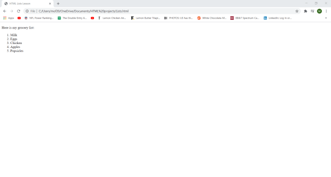
So, how did I create this list? First of all, I used the <p> tag for the “Here is my grocery list:” line. Next, to create my ordered list, I used the <ol> tag and for each list item, I used the <li> tag (I had to wrap each list item in its own <li> tag). In ordered lists, all list items are marked with numbers.

Next, I’ll show you how to create unordered lists:

<!DOCTYPE html>
<html lang="en" dir="ltr">
  <head>
    <meta charset="utf-8">
    <title>HTML Lists Lesson</title>
  </head>
  <body>
    <p>Here is the guest list for the party:</p>
    <ul>
      <li>Jessica</li>
      <li>Adam</li>
      <li>Michael</li>
      <li>Scott</li>
      <li>Allison</li>
      <li>Jacqueleine</li>
      <li><del>Matthew</del></li>
    </ul>
  </body>
</html>

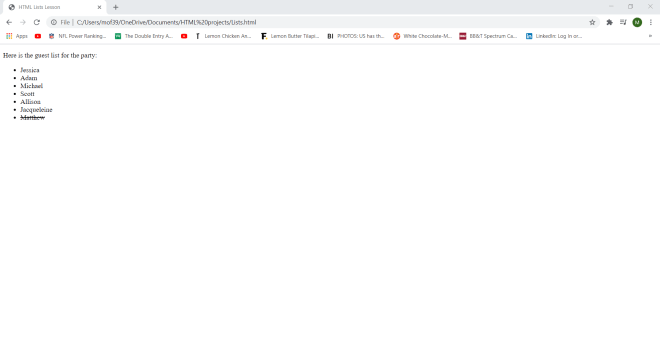
In this example, I used the <p> tag for the “Here’s the guest list for the party:” line. To create my unordered list, I used the same process I did for creating my ordered list, except I used the <ul> tag instead of the <ol> tag. Also, all of the elements in unordered lists are displayed with bullet points, not numbers.

  • Did you spot the call-back to the previous HTML lesson (the element in stroke-through)?

The third type of list you can create in HTML is the description list, which is a list of terms with a description of each term. Here’s how to create a description list in HTML:

<!DOCTYPE html>
<html lang="en" dir="ltr">
  <head>
    <meta charset="utf-8">
    <title>HTML Lists Lesson</title>
  </head>
  <body>
    <dl>
      <dt>Nashville, TN</dt>
      <dd>-Known as the "Music City"</dd>
      <dd>-Capitol of Tennessee</dd>
      <dd>-Famous for hot chicken</dd>
    </dl>
    <dl>
      <dt>Miami, FL</dt>
      <dd>-Warm weather all year long</dd>
      <dd>-Plenty of beaches</dd>
      <dd>-Area code is 305</dd>
    </dl>
  </body>
</html>

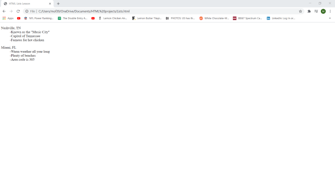
In this example, I have my two description lists each wrapped in a <dl> tag. For each list, I have the main term (Nashville, TN and Miami, FL) wrapped in a <dt> tag. Each description of each main term is wrapped in a <dd> tag (adding a dash after each item is optional).

Now, you’re probably wondering if it’s possible to create nested lists in HTML. The answer to that question is yes-here’s how to do so with an unordered list inside of an ordered list:

<!DOCTYPE html>
<html lang="en" dir="ltr">
  <head>
    <meta charset="utf-8">
    <title>HTML Lists Lesson</title>
  </head>
  <body>
      <ul>
        <li>Here are some of the greatest NBA players of all time:</li>
        <ol>
          <li>Shaquille O'Neal</li>
          <li>Kareem Abdul-Jabbar</li>
          <li>Lebron James</li>
          <li>Kobe Bryant</li>
          <li>Dwayne Wade</li>
          <li>Michael Jordan</li>
          <li>Charles Barkley</li>
          <li>Allen Iverson</li>
        </ol>
      </ul>
  </body>
</html>

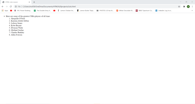
In this nesting example, the outermost list is the unordered list (tagged <ul>) while the innermost list is the ordered list (tagged <ol>). The unordered list only has one item while the ordered list has 8 items.

Now here’s a more complicated list nesting example, with an unordered list nested inside of an ordered list nested inside of an unordered list:

<!DOCTYPE html>
<html lang="en" dir="ltr">
  <head>
    <meta charset="utf-8">
    <title>HTML Lists Lesson</title>
  </head>
  <body>
      <ul>
        <li>Here are some of the greatest NBA players of all time:</li>
        <ol>
          <li>Shaquille O'Neal</li>
          <ul>
            <li>NBA Career: 1992-2011</li>
            <li>Teams: 6</li>
          </ul>
          <li>Kareem Abdul-Jabbar</li>
          <ul>
            <li>NBA Career: 1969-1989</li>
            <li>Teams: 2</li>
          </ul>
          <li>Lebron James</li>
          <ul>
            <li>NBA Career: 2003-present</li>
            <li>Teams: 3</li>
          </ul>
          <li>Kobe Bryant</li>
          <ul>
            <li>NBA Career: 1996-2016</li>
            <li>Teams: 1</li>
          </ul>
          <li>Dwayne Wade</li>
          <ul>
            <li>NBA Career: 2003-2019</li>
            <li>Teams: 3</li>
          </ul>
          <li>Michael Jordan</li>
          <ul>
            <li>NBA Career: 1984-1993, 1995-1998, 2001-2003</li>
            <li>Teams: 2</li>
          </ul>
          <li>Charles Barkley</li>
          <ul>
            <li>NBA Career: 1984-2000</li>
            <li>Teams: 3</li>
          </ul>
          <li>Allen Iverson</li>
          <ul>
            <li>NBA Career: 1996-2010</li>
            <li>Teams: 4</li>
          </ul>
        </ol>
      </ul>
  </body>
</html>

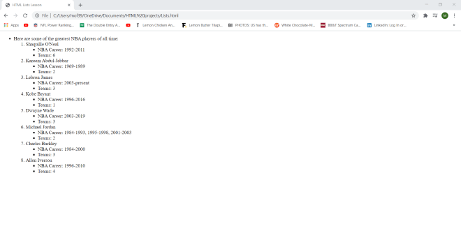
In this example, I didn’t change the outermost unordered list or the ordered list from the previous example. However, after each item in the ordered list, I added an unordered list with these two bullet points-NBA Career: and Teams: (which refer to the length of a player’s NBA career and how many teams he played for); since there are 8 items in the ordered list, I created 8 unordered lists nested within each of the ordered list items. Pretty neat if I do say so myself.

Thanks for reading,

Michael

Java Lesson 14: ArrayLists

Advertisements

Hello everybody,

Michael here, and today I’ll post a Java lesson-my first one in nearly six months! Today’s lesson will be on ArrayLists in Java. What exactly is an ArrayList? Well, here’s an example:

package lesson14;
import java.util.ArrayList;

public class ArrayListsDemo
{
public static void main (String[] args)
{
ArrayList<String> cities = new ArrayList<String>();
}
}

An ArrayList is basically a resizable array. See, in Java, you can’t add/remove elements from an array without creating a new array (which interestingly isn’t the case with Python arrays), but with ArrayLists, you can add and remove elements as you wish. The other differences between arrays and ArrayLists include:

  • You need to import a package for ArrayLists, but not for arrays.
  • The syntax for ArrayLists is different than that for arrays. Here’s the basic structure for ArrayLists:
    • ArrayList<type> name_of_array = new ArrayList <type>()
    • All elements in an ArrayList must be of the same type!

In the example above, the ArrayList is empty. Let’s see how we can fill it up:

package lesson14;
import java.util.ArrayList;

public class ArrayListsDemo
{
public static void main (String[] args)
{
ArrayList<String> cities = new ArrayList<String>();
cities.add(“Nashville”);
cities.add(“Franklin”);
cities.add(“Chattanooga”);
cities.add(“Knoxville”);
cities.add(“Memphis”);
cities.add(“Murfreesboro”);
cities.add(“Brentwood”);
System.out.println(cities);
}
}

And here’s the output:

run:
[Nashville, Franklin, Chattanooga, Knoxville, Memphis, Murfreesboro, Brentwood]
BUILD SUCCESSFUL (total time: 1 second)

In this example, I used the add method to add the names of Tennessee cities into the cities ArrayList. Unfortunately, there isn’t a way to add several elements into the ArrayList with just one line of code; you’ll need to add all of the elements 1-by-1.

Now that we have elements in our ArrayList, let’s see how we can access them:

System.out.println(cities.get(2));

run:
[Nashville, Franklin, Chattanooga, Knoxville, Memphis, Murfreesboro, Brentwood]
Chattanooga
BUILD SUCCESSFUL (total time: 1 second)

I would use the get method to access items in the cities ArrayList.  The same element accessing array logic applies to ArrayLists, meaning that the first element corresponds to index 0, the second to index 1, and so forth. If you’re wondering why you see the entire ArrayList again, that’s because I appended the line System.out.println(cities.get(2)) to the end of the code that was present.

OK, so what if we want to change an element? Well, here’s the line of code to do that (along with the resulting output):

cities.set(5, “Pigeon Forge”);
System.out.println(cities);

[Nashville, Franklin, Chattanooga, Knoxville, Memphis, Pigeon Forge, Brentwood]
BUILD SUCCESSFUL (total time: 8 seconds)

To change an element to an ArrayList, simply use the set method and include the index of the element you wish to change as well as the new value for that index as parameters. In this example, I am changing the element at index 5 (the 6th element) to Pigeon Forge.

Now let’s see how we can remove an element:

cities.remove(3);
System.out.println(cities);

[Nashville, Franklin, Chattanooga, Memphis, Pigeon Forge, Brentwood]
BUILD SUCCESSFUL (total time: 4 seconds)

To remove an element from an ArrayList, use the remove method along with the index of the element you want to remove as a parameter. In this example, I removed the element at index 3 (the 4th element).

  • If you wanted to empty the entire ArrayList, use the clear method.

Now let’s see how we can find the size of the ArrayList (after removing the element at index 3):

System.out.println(cities.size());

6

To find the size of the ArrayList, use the size method. In this example, the size of the cities ArrayList is 6.

Ok, so let’s see how we can loop through an ArrayList:

for (int i = 0; i < cities.size(); i++)
{
System.out.println(cities.get(i));
}

Nashville
Franklin
Chattanooga
Memphis
Pigeon Forge
Brentwood
BUILD SUCCESSFUL (total time: 5 seconds)

The best way to iterate through an ArrayList is with a for loop. Now, you could possibly try to iterate through an ArrayList with a while or do-while loop, but I’d stick with a for loop.

  • You should also use the size method to indicate how many times the loop should run.

You could also use a for-each loop to iterate through the ArrayList. Here’s how you’d write it:

for (String i: cities)

{

System.out.println(i);

}

Last but not least, I want to show you guys a cool little trick for ArrayLists that you can’t use for regular arrays. But first, you’d have to import the Collections class. Let me demonstrate:

import java.util.Collections;

Collections.sort(cities);
for (String i: cities)
{
System.out.println(i);
}

Brentwood
Chattanooga
Franklin
Memphis
Nashville
Pigeon Forge
BUILD SUCCESSFUL (total time: 2 seconds)

To sort the items in an ArrayList, first import java.util.Collections. To sort the elements, use the line Collections.sort(name of ArrayList) along with a for loop (or for-each loop, which I used here). You must loop through the ArrayList after sorting it, otherwise the sorting won’t work.

ArrayLists can either be sorted numerically or alphabetically (depending on the elements in your ArrayList). From what I tried, it seems like the Collections.sort method can only sort either in ascending order (for numerical ArrayLists) or alphabetical order (for non-numerical ArrayLists). I’m not sure if ArrayLists can be sorted in descending numerical order or reverse alphabetical order, but then again there could be methods for accomplishing these types of sorts.

Thanks for reading,

Michael

Python Lesson 9: Nested Lists and Tuples

Advertisements

Hello everybody,

It’s Michael, and today’s post will be about nesting. This post will involve lists, tuples, sets, and dictionaries, but it won’t necessarily be a continuation of my last two Python posts. In this post, I’ll be demonstrating nested and tuples (with the next post covering nested sets and dictionaries).

First I will demonstrate a nested list (think of this as a list-within-a-list):

fruitsandveggies = [‘bananas’, ‘oranges’, [‘peppers’, ‘celery’, ‘zucchini’,], ‘apples’
, ‘strawberries’]

And here’s some sample output (based on me choosing a specific element from the nested list):

print(fruitsandveggies[2][1])

celery

In this example, I have the nested list fruitsandveggies and have selected element [2][1] from the list. However, you’re probably wondering what element I’m referring to when I say [2][1]. In this list, [2] refers to the outermost list while [1] refers to the innermost list. So when I want to pick element [2][1] from the fruitsandveggies list, I’m saying that I want to pick index 2 (the 3rd item) from the outermost list and index 1 (the 2nd item) from the innermost list (the corresponding element is celery).

So whenever you see something like fruitsandveggies[2][1], remember that the first index ([2] in this case) represents the outermost list and any subsequent indexes represent lists that are further inward. In this example, [1] would represent a list that is further inward. Had I included more nested lists, any subsequent indexes would’ve represented lists that were further inward. The last index listed would represent the innermost list.

So remember that when you see something like list name[a][b][c][d][e], remember that the first index listed (represented by [a]) would represent the main list. Any subsequent indexes (represented by [b], [c], and [d])  represent lists that are further inward, while the last index (represented by [e])  represents the innermost list.

  • Helpful tip-when you are selecting an element from a nested list, remember to choose an index with a nested list! For instance, a statement like print(fruitsandveggies[3][1])​  wouldn’t have worked because index 3 (the 4th item in the outermost list) doesn’t contain a nested list.

You can also do many of the same things with nested lists that you can with normal lists, such as:

…negative indexing

fruitsandveggies = [‘bananas’, ‘oranges’, [‘peppers’, ‘celery’, ‘zucchini’], ‘apples’
, ‘strawberries’]

print(fruitsandveggies[-3][-1])

zucchini

Remember that the negative indexing rules that apply for regular lists also apply for nested lists (e.g. first index in negative indexing is -1, not 0)

…adding items to the list (using the same methods you would use for regular lists)

fruitsandveggies.append(‘grapefruit’)
fruitsandveggies.insert(2, ‘squash’)

print(fruitsandveggies)

[‘bananas’, ‘oranges’, ‘squash’, [‘peppers’, ‘celery’, ‘zucchini’], ‘apples’, ‘strawberries’, ‘grapefruit’]

In this example, I used append to add the item grapefruit to the list and insert to add squash to the list.

When using these methods with nested lists, keep in mind that the appended item will be added to the outermost list, not any nested lists. Also keep in mind that when you use the insert method in a nested list, the index you want to place the element in corresponds to the outermost list, not any nested lists. In this example, I wanted to insert the element squash at index 2; this means that squash would be inserted at index 2 OF THE OUTERMOST LIST.

…removing items from the list (using the same methods that work for normal lists):

fruitsandveggies.pop()
del fruitsandveggies[2][1]

print(fruitsandveggies)

[‘bananas’, ‘oranges’, [‘peppers’, ‘zucchini’], ‘apples’]

In this example, I used the pop and del methods to remove items from the list fruitsandveggies. Pop removed the last item from this list; however, it might have removed a different element had I specified an element to remove. Del removed the item from this last that was located at the index I specified- [2][1] (meaning that the item at index 1 of the nested list was removed).

…finding the length of a list:

fruitsandveggies = [‘bananas’, ‘oranges’, [‘peppers’, ‘celery’, ‘zucchini’], ‘apples’
, ‘strawberries’]

print(len(fruitsandveggies[1]))
print(len(fruitsandveggies[2]))

7
3

Finding the length of a nested list is essentially the same as finding the length of a regular list (you would also use the len method), but include an index after the list name. The index will let Python know the list whose length you wish to find. For instance, if you use the index [1], you will get the length of the entire list (which in this case is 7). However, if you were to use the index [2], you would get the length of the nested list (which in this case is 3) . If I had more nested lists in this example,  I would use indexes such as [3], [4], [5], and so on, depending on how far inward the lists were located.

Last but not least, let’s see how we can iterate through the elements of a nested list:

for list in fruitsandveggies:
for i in list:
print(fruitsandveggies)

[‘bananas’, ‘oranges’, [‘peppers’, ‘celery’, ‘zucchini’], ‘apples’, ‘strawberries’]
[‘bananas’, ‘oranges’, [‘peppers’, ‘celery’, ‘zucchini’], ‘apples’, ‘strawberries’]
[‘bananas’, ‘oranges’, [‘peppers’, ‘celery’, ‘zucchini’], ‘apples’, ‘strawberries’]
[‘bananas’, ‘oranges’, [‘peppers’, ‘celery’, ‘zucchini’], ‘apples’, ‘strawberries’]
[‘bananas’, ‘oranges’, [‘peppers’, ‘celery’, ‘zucchini’], ‘apples’, ‘strawberries’]
[‘bananas’, ‘oranges’, [‘peppers’, ‘celery’, ‘zucchini’], ‘apples’, ‘strawberries’]
[‘bananas’, ‘oranges’, [‘peppers’, ‘celery’, ‘zucchini’], ‘apples’, ‘strawberries’]
[‘bananas’, ‘oranges’, [‘peppers’, ‘celery’, ‘zucchini’], ‘apples’, ‘strawberries’]
[‘bananas’, ‘oranges’, [‘peppers’, ‘celery’, ‘zucchini’], ‘apples’, ‘strawberries’]
[‘bananas’, ‘oranges’, [‘peppers’, ‘celery’, ‘zucchini’], ‘apples’, ‘strawberries’]
[‘bananas’, ‘oranges’, [‘peppers’, ‘celery’, ‘zucchini’], ‘apples’, ‘strawberries’]
[‘bananas’, ‘oranges’, [‘peppers’, ‘celery’, ‘zucchini’], ‘apples’, ‘strawberries’]
[‘bananas’, ‘oranges’, [‘peppers’, ‘celery’, ‘zucchini’], ‘apples’, ‘strawberries’]
[‘bananas’, ‘oranges’, [‘peppers’, ‘celery’, ‘zucchini’], ‘apples’, ‘strawberries’]
[‘bananas’, ‘oranges’, [‘peppers’, ‘celery’, ‘zucchini’], ‘apples’, ‘strawberries’]
[‘bananas’, ‘oranges’, [‘peppers’, ‘celery’, ‘zucchini’], ‘apples’, ‘strawberries’]
[‘bananas’, ‘oranges’, [‘peppers’, ‘celery’, ‘zucchini’], ‘apples’, ‘strawberries’]
[‘bananas’, ‘oranges’, [‘peppers’, ‘celery’, ‘zucchini’], ‘apples’, ‘strawberries’]
[‘bananas’, ‘oranges’, [‘peppers’, ‘celery’, ‘zucchini’], ‘apples’, ‘strawberries’]
[‘bananas’, ‘oranges’, [‘peppers’, ‘celery’, ‘zucchini’], ‘apples’, ‘strawberries’]
[‘bananas’, ‘oranges’, [‘peppers’, ‘celery’, ‘zucchini’], ‘apples’, ‘strawberries’]
[‘bananas’, ‘oranges’, [‘peppers’, ‘celery’, ‘zucchini’], ‘apples’, ‘strawberries’]
[‘bananas’, ‘oranges’, [‘peppers’, ‘celery’, ‘zucchini’], ‘apples’, ‘strawberries’]
[‘bananas’, ‘oranges’, [‘peppers’, ‘celery’, ‘zucchini’], ‘apples’, ‘strawberries’]
[‘bananas’, ‘oranges’, [‘peppers’, ‘celery’, ‘zucchini’], ‘apples’, ‘strawberries’]
[‘bananas’, ‘oranges’, [‘peppers’, ‘celery’, ‘zucchini’], ‘apples’, ‘strawberries’]
[‘bananas’, ‘oranges’, [‘peppers’, ‘celery’, ‘zucchini’], ‘apples’, ‘strawberries’]
[‘bananas’, ‘oranges’, [‘peppers’, ‘celery’, ‘zucchini’], ‘apples’, ‘strawberries’]
[‘bananas’, ‘oranges’, [‘peppers’, ‘celery’, ‘zucchini’], ‘apples’, ‘strawberries’]
[‘bananas’, ‘oranges’, [‘peppers’, ‘celery’, ‘zucchini’], ‘apples’, ‘strawberries’]
[‘bananas’, ‘oranges’, [‘peppers’, ‘celery’, ‘zucchini’], ‘apples’, ‘strawberries’]
[‘bananas’, ‘oranges’, [‘peppers’, ‘celery’, ‘zucchini’], ‘apples’, ‘strawberries’]
[‘bananas’, ‘oranges’, [‘peppers’, ‘celery’, ‘zucchini’], ‘apples’, ‘strawberries’]
[‘bananas’, ‘oranges’, [‘peppers’, ‘celery’, ‘zucchini’], ‘apples’, ‘strawberries’]
[‘bananas’, ‘oranges’, [‘peppers’, ‘celery’, ‘zucchini’], ‘apples’, ‘strawberries’]

In this example, I iterated through this nested list with a nested for loop. One thing I didn’t realize when I created this loop was that the list was going to be printed 21 times (I’m guessing it’s 21 times because there are 7 elements in the main list while there are three elements in the nested list, so 7 * 3 = 21).

Next, I will demonstrate nested tuples. But first, let me show you how to create a nested tuple, as the process isn’t as simple as the one for creating a nested list:

tuple1 = (1, 3, 5, 7, 9)
tuple2 = (0, 2, 4, 6, 8)
tuple3 = tuple1, tuple2
print(tuple3)

((1, 3, 5, 7, 9), (0, 2, 4, 6, 8))

See, with a nested list, all you would need to do is write a list-within-a-list (or several lists-within-lists). On the other hand, with a nested tuple, you would actually need to create a new tuple that concatenates your other tuples, as I did in the above example (and yes, you can use a comma to concatenate your tuples. This is not Java).

Now, let’s say we wanted to access an item in our nested tuple. How do we do that?:

print(tuple3[1][1])

2

The process for accessing an item in a nested tuple is the same as it is for accessing an item in a nested list-use multiple indexes to get the element you want. However, the way indexes are counted in nested tuples differs from the index counting in nested lists, as individual tuples-within-the-tuple are counted as individual indexes. For instance, in tuple3, the first tuple (tuple1) counts as index 0 while the second tuple (tuple2) counts as index 1.

But what if I had only used a single index? Let’s see what would happen:

print(tuple3[1])

(0, 2, 4, 6, 8)

In this example, I used a single index-[1]-and got the entire second tuple as a result.

  • Remember that if you want to get a single tuple element, use multiple indexes. If you want to get a whole tuple, use a single index.

Negative indexing also works with nested tuples. Here’s an example (using both single and multiple indexes):

print(tuple3[-1])

(0, 2, 4, 6, 8)

print(tuple3[-1][-3])

4

How would we iterate through a nested tuple? We would basically use the same process we use to iterate through regular tuples:

for i in tuple3:
print(i)

(1, 3, 5, 7, 9)
(0, 2, 4, 6, 8)

Interestingly, the tuples printed out separately-by this I mean the tuples-within-the-tuple are displayed on separate lines rather than on the same line separated by a comma.

Now, how would we find the length of a nested tuple? Let’s find out:

print(len(tuple3))

2

How did I get 2 instead of 10? In this example, Python counted each individual tuple-tuple1 and tuple2-inside of my large tuple-tuple3-as an individual element. Since there are two tuples-within-the-tuple, len returned 2.

You may have noticed that I didn’t mention anything about adding or removing elements from nested tuples. This is because the methods that work for adding and removing items from regular tuples won’t work for nested tuples.

Thanks for reading,

Michael


Python Lesson 7: Lists & Tuples

Advertisements

Hello everybody,

It’s Michael, and this post will be the first in a new series of Python posts. Today’s Python post will cover lists and tuples.

List and tuples are two of the four major collection types in Python (sets and dictionaries being the other two), but what are the differences between them?:

  • Lists are ordered and changeable; duplicates are allowed
  • Tuples are ordered but unchangeable; duplicates are also allowed
  • Dictionaries are unordered but changeable and indexed; no duplicates here
  • Sets are unordered and unindexed; no duplicates here

Still stumped about lists, tuples, dictionaries, and sets? Don’t worry, I’ll explain lists and tuples in today’s posts (I’ll explain dictionaries and sets in the next post).

I’ll start with lists. Here is a very simple example:

This list contains the names of three states. Notice anything else familiar?

If you were thinking of the square brackets, you are correct. See, arrays in Python (and Java for that matter) also use square brackets. Also, by the way lists are structured, you might’ve thought they were arrays (and Python lists and arrays are very easy to mix up with each other).

So how do lists and arrays differ from each other? Here are three ways:

  • Arrays have to be declared while lists don’t (recall that, more often than not, you won’t need to declare variable types in Python) since lists are automatically recognized as such by Python.
  • While lists work fine storing many different data types, if you need to do arithmetic functions on a series of elements, you’re better off using arrays.
  • Arrays store data more compactly and efficiently than lists, so if you’ve got lots of elements (like tens of thousands of elements), you’re betting off storing them in an array.

How do you extract elements from a list? It’s pretty much the same way you would with an array:

As you can see from this list, you would extract an element in a list by writing list name[list element]. You can use either a print or return statement to print the element you are looking for, but don’t use both.

  • Remember that, like with arrays in Java, lists start at element 0, so when I picked element 2 from the list, I was really choosing the third item in the list, not the second.

The example I just showed you is a really basic example as to what a list can do. You can also select a range (or ranges) of elements in lists, just as you can with arrays in Java. Here’s an example:

In this example, I selected elements 1-3 from the stores list. But how come only two elements were printed? When you are selecting elements for a range, the last element is excluded. In other words, the lower bound listed in the range (1 in this example) will be included but the upper bound for the range (3 in this example) won’t be included. The range will only display elements from the lower bound to the upper bound-1 (2 in this example).

But wait, there’s another way to select elements from a list in Python. It’s called negative indexing and here are two examples of that (the first showing an individual element selection and the second showing a range:

Negative indexing is essentially the reverse of regular indexing, as the first index is the last item in the list and the last index is the first item in the list. Also keep in mind that the last item in the list corresponds to index -1 because after all, there is no -0.

When choosing ranges in negative indexing, the same upper bound/lower bound logic that applies to regular indexing also applies here. Even though you have an upper bound and lower bound, the lower bound will be displayed but the upper bound won’t be displayed. Rather, the element BEFORE the element in the upper bound will be the last element displayed.

One more thing regarding choosing ranges in lists that I wanted to mention is that, whether using negative indexing or regular indexing, you don’t need both an upper or lower bound (but you can’t have neither, because that’s not a range). Here are two examples (the first using regular indexing and the second using negative indexing):

In the first print statement in the regular indexing example, everything from index 2 (3rd item in the list) onwards is printed. In the second print statement, everything up until BUT NOT INCLUDING index 3 (4th element) is printed.

In the first print statement in the negative indexing example, everything beyond BUT NOT INCLUDING index -2 (5th item in the list) is printed. In the second print statement, everything from index -4 (3rd item in the list) onwards is printed.

OK, now that I’ve discussed selecting items from lists, let’s now talk about modifying lists.

The first thing I want to discuss is changing elements in lists. Here’s an example:

In this list, I changed index 4 (the 5th item in the list) to Captain Marvel then printed out the new list with the changed index. If you want to change an element in a list, here is the syntax for doing so:

  • List name [list index you want to change] = new element for that index

Now let’s talk about adding items to a list. In Python, there are two methods for accomplishing this-append and insert. Both methods add items to list, but append will only add items to the end of a list while insert will add items at any position in the list (so long as you specify the position where you would like to add an item). Here’s an example of each method in action (along with the new list after each method is executed):

In this example, I appended Thor The Dark World to the list as well as added Spider-Man Homecoming to the list at index 2 (which is the 3rd element).

Now, what should we do if we want to remove items from a list? There are three possible methods for doing so-remove, pop, and del. Remove will remove a specified item from the list, pop will removed a specific index (which corresponds to a specific item) from the list-or the last index if an index isn’t specified, and del will also remove a specific index.

  • Keep in mind that when using del, you must specify an index, but you don’t have to specify an index if you’re using pop.

Now, here’s an example of the remove, pop, and del methods in action, along with the resulting list (keep in mind that this list is building from the list in the previous example):

In this list, I removed the element Captain Marvel, popped off the last element of the list (since I didn’t specify an element to pop off, pop will automatically remove the last element of the list), and deleted index 1 (the 2nd element) of the list.

The last thing I want to discuss about lists is how you can see whether or not an element is in a list. Here’s an example of this:

In this example, I am checking to see whether or not Avengers Infinity War is in the list MARVEL (the list I made from concatenating MCU and nonMCU). Depending on whether Avengers Infinity War is in the list MARVEL, one of two messages will appear-either Infinity War is in this list or Infinity War isnt in this list. Since the aforementioned element wasn’t in the list MARVEL, the message Infinity War isnt in this list is printed.

  • Jupyter notebook indents the bodies of if-else statements, loops, and functions (which I’ll discuss in a future lesson). Spyder doesn’t do this.

Last but not least, let’s see how we can find the length of a list:

To find the length of a list, simply write len (name of list). That’s it.

Now that I’ve discussed everything I wanted to discuss about lists, let me move on to tuples.

Tuples are similar to lists since both are ordered collections of items. However, tuples are written with round, not square, brackets, and unlike lists, they are unchangeable, which means you can’t modify the tuple in any way.

One great example of tuples is the coordinate plane (the one you were likely first introduced to in school). The coordinate plane is full of tuples, such as (3,2), (2,7), and (-1 5), just to name a few.

Now, let’s first see how we can access tuple items:

Notice anything familiar? If you do, it’s because you would access a tuple item the same way you would a list item. However, you must write print before the part where you access the tuple item, since tuples aren’t callable on their own (and I got an error message when I tried to execute the statement vegetables[1])

Now, how would we use negative indexing in a tuple? Let’s take a look:

As it turns out, negative indexing with a tuple is the same as negative indexing with a list. Just remember to write print before the part where you access the tuple item.

Now, how would we select a range of items in a tuple (using both regular and negative indexing):

Well what do you know? Selecting ranges of items in tuples is the same as selecting ranges of items in lists. Even the same inclusion/exclusion rules apply-by that I mean the index corresponding to the lower bound (1 and -3 in this example) will be included in the output while the index corresponding to the upper bound (4 and -1 in this example) will be excluded.

Now, how would be change an item in a tuple? Let’s find out:

Yeah, you can’t change items in a tuple-this was basically a trick question (I did mention that tuples were unchangeable at the beginning of this post).

But, there is a workaround for this. Here’s how that would work:

I first converted the vegetables tuple into a list, which is referred to as vegetables2. I then changed index 2 in vegetables2 to zucchini, converted vegetables2 back into the original vegetables tuple, and printed the new vegetables tuple.

So if you ever need to do something like this, here’s how to change an item in a tuple:

  • Turn tuple into list
  • Change element in list
  • Turn list back into tuple

Now, how would we add or remove items from a tuple? Let’s find out:

  • Keep in mind that I’m trying to add an item on the first line but trying to remove an item on the second line.

OK, I’ll admit this was a total trick question. Tuples are unchangeable, meaning that you can’t add or remove elements from tuples.

You can, however, delete a tuple completely using the syntax del name_of_tuple.

Now, let’s see how we can join-or concatenate-two tuples together:

In this example, I made a new tuple fruits which I joined with the vegetables tuple to make the fruitsandvegetables tuple, which I then printed out.

Next up-let’s see how we can check whether or not an item is in a tuple:

The process for checking whether an item is in a tuple is identical to the process for checking whether an item is in a list (though an else statement isn’t necessary).

Let’s next look at iterating through a tuple with a for loop:

The process for iterating through a tuple with a for loop is the same as the iteration process with a for loop for a list.

Last but not least, let’s see how we check the length of our tuple:

Simply using the len method (along with the name of the tuple) will allow you to check the length of the tuple.

Thanks for reading,

Michael


Java Program Demo 2: Arrays, Random Numbers, Inheritance & Polymorphism

Advertisements

Hello everybody,

It’s Michael, and today’s post will be my second Java program demo. I will focus on the topics of the last 3 posts (random number generators, arrays, inheritance, and polymorphism); however I may also utilize concepts from the first six Java lessons (such as for loops and if statements) since Java concepts build on each other.

In this demo, I will create three programs that demonstrate the concepts from Java Lessons 7-9 (with some concepts from Lessons 1-6 as well).

Here is my first program:

package programdemo2;
import java.util.Random;

public class ProgramDemo2
{
public static void main(String[] args)
{
String [] maleNames = {“Alex”, “Brian”, “Chester”, “David”, “Eric”, “Felipe”, “Gabriel”,
“Henry”, “Ike”, “Jacob”, “Kyle”, “Lenny”, “Michael”, “Nicholas”,
“Oliver”, “Phillip”, “Quentin”, “Ricky”, “Steven”, “Todd”,
“Ulises”, “Victor”, “William”, “Xavier”, “Yancy”, “Zach”};

Random gen = new Random ();
int limit = gen.nextInt(25);

System.out.println (maleNames[limit]);
}

}

This program demonstrates a simple one-dimensional array along with a random number generator. The array shown above is a String array containing random males names for all 26 letters of the alphabet (and yes Yancy is an actual male name). The random number generator’s upper limit is set to 25, since there are 26 elements (remember the “indexes start at 0” rule). The system will print out any one of the 26 names mentioned (at random). Let’s check out two sample outputs:

run:
Jacob
BUILD SUCCESSFUL (total time: 2 seconds)

run:
William
BUILD SUCCESSFUL (total time: 0 seconds)

Our two sample outputs-Jacob and William-correspond to indexes 9 and 22, respectively (or the 10th and 23rd elements in the array).

Now let’s demonstrate a two-dimensional array:

package programdemo2;
import java.util.Scanner;

public class ProgramDemo2
{

public static void main(String[] args)
{
Scanner s = new Scanner (System.in);
System.out.println(“Pick a number: “);
int num = s.nextInt();

int [][] multiples = new int [5][5];

for (int i = 0; i <= 4; i++)
{
for (int j = 0; j <= 4; j++)
{
multiples[i][j] = num*(i+1);
}

}

System.out.println (multiples[4][4]);
}
}

Using a combination of a Scanner, a for-loop, and a two-dimensional array, this program will create a two-dimensional five-by-five array based on the number you input into the Scanner. The five rows will contain five different numbers, while the five columns will contain the same number through the column. The number in a column is calculated using the formula num*(I+1), which means that the number inputted into the Scanner will be multiplied by I+1 in order to figure out what number goes into the column. Remember that I increments by one after each loop iteration, so when the loop starts at 0, the number inputted will be multiplied by 1 (since I+0 would be 1). Likewise, on the final iteration of the loop (I=4), the inputted number will be multiplied by 5, since 4+1=5.

Let’s create a sample array, using 4 different outputs (and using 6 as the Scanner number each time):

run:
Pick a number:
6
30
BUILD SUCCESSFUL (total time: 5 seconds) index[4][2]

run:
Pick a number:
6
24
BUILD SUCCESSFUL (total time: 5 seconds) index[3][3]

run:
Pick a number:
6
24
BUILD SUCCESSFUL (total time: 2 seconds)index[3][0]

run:
Pick a number:
6
12
BUILD SUCCESSFUL (total time: 6 seconds)index[1][2]

In each of these four outputs, I use a different index but the same Scanner number-6. The indexes to which these outputs correspond are mentioned to the right of the BUILD SUCCESSFUL line.

Here’s a visualization of the array with the outputs filled in. With the information given in the program and outputs, could you fill in the missing elements?

My last program demo will involve polymorphism and inheritance. Here is my main class (the one from which I will run the program):

import java.util.Scanner;

public class ProgramDemo
{
public static void main (String[]args)
{
Scanner s = new Scanner (System.in);
System.out.println(“Pick a number: “);
double num = s.nextDouble();

String [] time = {“hours”, “days”, “weeks”, “months”};

System.out.println(“Pick an index from 0-3:”);
int index = s.nextInt();

if (index == 0)
{
Days d = new Days();
d.measure(num);
}

else if (index == 1)
{
Weeks w = new Weeks ();
w.measure(num);
}

else if (index == 2)
{
Months m = new Months ();
m.measure(num);
}

else if (index == 3)
{
Years y = new Years ();
y.measure(num);
}

else
{
System.out.println(“Pick another number”);
}
}
}

Now here’s my superclass (which is NOT the same as my main class):

public class TimeMeasurements extends ProgramDemo
{
public void measure ()
{
double num = 0;
System.out.println(num);
}
}

And here are my four subclasses:

public class Days extends TimeMeasurements
{
public void measure(double num)
{
System.out.println(“Number of days is: ” +num/24);
}
}

public class Weeks extends TimeMeasurements
{
public void measure (double num)
{
System.out.println (“Number of weeks is: ” + num/7);
}
}

public class Months extends TimeMeasurements
{
public void measure (double num)
{
System.out.println (“Number of months is: ” + num/4);
}
}

public class Years extends TimeMeasurements
{
public void measure (double num)
{
System.out.println (“Number of years is: ” +num/12);
}
}

Before I get into sample outputs, let me explain the structure of my program.

The first line of the main program in the main method creates a Scanner object, which I will use to store the double variable num. After the line asking the user for input, there is a String array called time, which contains four elements-hours, days, weeks, and months. The user is then asked to choose a number from 0-3 (corresponding to each of the possible indexes), and based on the input, one of the four if statements will execute. OK, there’s also an else statement, but that will only execute if the number you pick for the Pick an index from 0-3:  line is not between 0 and 3 (or any decimals for that matter).

The superclass TimeMeasurements extends the main class ProgramDemo; this means that TimeMeasurements inherits all variables and methods of the ProgramDemo class. This extension ultimately doesn’t mean much since the only method in ProgramDemo is the default main method; however, the num variable from ProgramDemo does carry over.

Here is where polymorphism comes in. In TimeMeasurements, there is a method called measure which converts a number from one unit of time to another. This method is of type void-meaning it doesn’t have a return statement-but its parameter is double num, which is the exact same variable and type as the double num in my main class. Each of my four subclasses-Days, Weeks, Months, and Years-also contains the measure method, but each class will return a different result for the same method. Days divides num by 24 since I’m converting from hours to days. Weeks divides num by 7, Months divides num by 4, and Years divides num by 12. The polymorphism is present throughout the measure method in my superclass and subclasses since the calculations in each method differ from class to class (and the TimeMeasurements class simply sets the num to 0).

  • My subclasses extends the superclass TimeMeasurements, which in turn extends the main class ProgramDemo. So in turn, my 4 subclasses extend ProgramDemo
    • This is why I chose to use num as the variable for all 4 subclasses and TimeMeasurements; using num would allow the program to produce output based on the formulas specified in each of the subclasses measure methods.
  • I used double for num because chances are high that the program’s calculations will involve decimals.
  • A method’s parameters and type don’t have to be the same. Case in point-the measure method; this method is of type void but the parameter is of type double.

There are 4 if statements and an else statement in this program, which will do the following based on the Pick an index input:

  • If 0 is chosen, an object of class Day will be created and the measure method for class Day will be executed. The output will show you how many days are in X amount of hours (X being your num input).
  • If 1 is chosen, an object of class Week will be created and the measure method for class Week will be executed. The output will show you how many weeks are in X days.
  • If 2 is chosen, an object of class Month will be created and the measure method for class Month will be executed. The output will show you how many months are in X weeks.
  • If 3 is chosen, an object of class Year will be created and the measure method for class Year will be executed. The output will show you how many years are in X months.
  • If neither 0, 1, 2, or 3 is chosen, the else statement will execute, which will simply display the line Pick another number.

Now let’s show five sample outputs (to account for the 5 possible conditions). For the outputs, I’ll go in order of conditional statements (in other words, I’ll start with 0):

run:
Pick a number:
65
Pick an index from 0-3:
0
Number of days is: 2.7083333333333335
BUILD SUCCESSFUL (total time: 49 seconds)

In this output, I chose index 0 and the number 65-referring to 65 hours. The numerical output was 2.71 (rounded to 2 decimal places), meaning that there are approximately 2.71 days in 65 hours.

Next I’ll choose index 1:

run:
Pick a number:
112
Pick an index from 0-3:
1
Number of weeks is: 16.0
BUILD SUCCESSFUL (total time: 13 seconds)

I chose 112 as my num input-referring to 112 days. I got 16 as the output, which means that 112 days equals 16 weeks.

Now I’ll use index 2:

run:
Pick a number:
88
Pick an index from 0-3:
2
Number of months is: 22.0
BUILD SUCCESSFUL (total time: 23 seconds)

I chose 88 as my num input-referring to 88 weeks. I got 22 as the output, which means that 88 weeks equals 22 months.

Now time to try index 3:

run:
Pick a number:
105
Pick an index from 0-3:
3
Number of years is: 8.75
BUILD SUCCESSFUL (total time: 10 seconds)

And last but not least, let’s enter a number other than 0, 1, 2, or 3:

run:
Pick a number:
35
Pick an index from 0-3:
5
Pick another number
BUILD SUCCESSFUL (total time: 8 seconds)

I picked 35 as my number and 5 as my index and, since my chosen index wasn’t 0, 1, 2, or 3, I got the message Pick another number as my output.

Thanks for reading,

Michael

Java Lesson 8: Arrays

Advertisements

Hello everybody,

It’s Michael, and today’s Java post will be about arrays. But what exactly do arrays do in Java?

Arrays are basically a list of variables that are referred to by a common name. Here’s an example:

Florida Ohio Georgia Mississippi Texas Montana

This is an array of states, which I will call states.

You can make arrays for variables of any Java type, including:

  • int
    • And any numerical type for that matter (i.e. double, float)
  • char
  • boolean
  • String

However, you cannot have several variable types in an array (so no mixing String elements with int elements). For instance, if you wanted to include 737 Down Over ABQ in your array, the 737 would have to be a String in order to make the array work (assuming Down Over ABQ are all String).

Now let me demonstrate a simple array program:

package javalessons;

public class JavaLessons
{

public static void main(String[] args)
{
String [] stateCaps = {“Helena”, “Salem”, “Tallahassee”, “Atlanta”, “St.Paul”, “Pierre”, “Columbus”, “Providence”};
System.out.println(stateCaps[4]);
}
}

And here are two sample outputs (using a different index for each array):

run:
Tallahassee
BUILD SUCCESSFUL (total time: 0 seconds)

run:
St.Paul
BUILD SUCCESSFUL (total time: 0 seconds)

The first thing I did in the program is to create my array declaration-String [] stateCaps = {"Helena", "Salem", "Tallahassee", "Atlanta", "St.Paul", "Pierre", "Columbus", "Providence"}. The point of the array declaration is to create an array and POSSIBLY fill it with elements.

I say POSSIBLY because there are three ways I can go about create my array and filling it with elements. Here are some possibilities:

  • Do what I did in the aforementioned program, which is to create the array and the elements in the same line of code (separated by an equals sign)
  • Create the array and allocate space to the array in the same line, which would mean I would have written String [] stateCaps = new String [8] to create a String array with 8 values. Meanwhile, I would have added elements in 8 separate lines of code, starting with stateCaps[0]="Helena" and continuing on until I fill the array.
  • Create a for loop. More on that later in this post.

OK, here’s something I want to mention about that second bullet point. Each element in an array is called an index (plural: indices). However, the first index in an array is [0] not [1] since array indices are counted starting from 0, not 1. So the first index in an array is [0], the second index is [1], the third index is [2], and so on.

In each of my outputs, I chose a different index, and thus got a different output each time. The first output-Tallahassee-corresponds to index 2-or the third element in the array, which is “Tallahassee”. The second output-St.Paul-corresponds to index 4-or the fifth element in the array, which is “St.Paul”.

Next, remember how I mentioned that you could use a random number generator in arrays in my previous post? Here’s how you can do that (using a different array):

package javalessons;
import java.util.Random;

public class JavaLessons
{

public static void main(String[] args)
{
String [] cartoons = {“Family Guy”, “Spongebob”, “Simpsons”, “South Park”,
“Archer”, “Daniel Tiger’s Neighborhood”, “Arthur”, “Looney Tunes”,
“Big Mouth”, “Rick & Morty”};
Random gen = new Random ();
int index = gen.nextInt(9);

System.out.println(cartoons[index]);
}
}

And here are two sample outputs:

run:
Big Mouth
BUILD SUCCESSFUL (total time: 0 seconds)

run:
Spongebob
BUILD SUCCESSFUL (total time: 2 seconds)

In this program, I first imported java.util.Random, which is what you need to do if you plan on using a random number generator in your program. I also remembered to create Random and int variables, which you need to do in order to have a random number generator handy and, in the case of the int variable, set the upper limit for the random number generator. In this case, the upper limit for my generator is 9, since there are 10 elements in my array (remember array elements start counting from 0). Had I used 10 as the upper limit, there is a chance I would have gotten an error message since there is no index 10. I then created an array-cartoons-and filled it with 10 elements (10 American cartoons).

For my output, I asked the program to print out a random element each time I run the program. In my first sample output, index 8 was displayed (corresponding to Big Mouth) while in my second output, index 1 was displayed (corresponding to Spongebob).

Now let me show you how to fill in an array using a for loop:

package javalessons;

public class JavaLessons
{

public static void main(String[] args)
{
int [] multiples = new int [15];

for (int i = 0; i <= 14; i++)
{
multiples[i]=i*8;
}

System.out.println (multiples[3]);
}
}

And here are two sample outputs (each using a different index):

run:
24
BUILD SUCCESSFUL (total time: 1 second)

run:
48
BUILD SUCCESSFUL (total time: 0 seconds)

This program demonstrates a very simple way to fill in an array using a for loop. I used my for loop to fill in my array with multiples of 8, hence the I*8. I first created my array in the line directly above the for loop, then I created the for loop to fill my array with elements. In my for loop, I started my counter at 0 (remember that array indices start from 0), asked it to stop at 14 (since I will have 15 elements in my array), and asked it to increment by 1 after each iteration.

  • I’ll admit that the new int [15] may seem redundant since I already determined that my loop will have 15 iterations (and thus 15 elements).

My sample outputs printed indexes 3 and 6 (the 4th and 7th elements respectively), which correspond to the numbers 24 and 48. Remember that since I started this loop with 0, the first element will be 0, since 0 times 8 is 0.

Last but not least, I will introduce the concept of two dimensional arrays using a combination of a for loop and a random number generator. Here’s a sample program:

package javalessons;
import java.util.Random;

public class JavaLessons
{

public static void main(String[] args)
{
int [] [] twoDim = new int [6][6];
Random gen = new Random ();
int boundary = gen.nextInt(35);

for (int i = 0; i <= 5; i++)
{
for (int j = 0; j <= 5; j++)
{
twoDim [i][j] = boundary;
}
}

System.out.println (twoDim[2][3]);
}
}

And here are two sample outputs:

run:
24
BUILD SUCCESSFUL (total time: 0 seconds)

run:
1
BUILD SUCCESSFUL (total time: 1 second)\

The process of working with two-dimensional arrays (or other multidimensional arrays for that matter) is a little different than the process of working with one dimensional arrays. First of all, you would need a nested for loop (or a for loop within a for loop) to traverse through (and possibly fill in) your array. Second, you would need two squares [] [] to initialize the array as opposed to just one [].

  • You don’t always need a nested for loop to fill in a two dimensional array. Plus if you are dealing with non-numerical elements like String, a loop isn’t very practical to use.
  • Here’s another way to fill in a 2-dimensional array, using String elements:
    • Let’s say our array is 3 by 3.
    • This is another way to fill in elements:
      • String [][] cities = {{"Fort Collins", "Mentor", "Miami"}, {"Bozeman", "Annapolis", "Pittsburgh"}, {"Boston", "Omaha", "Manhattan"}}
      • Since this array is 3 by 3, we would have 3 groups of 3 elements each.
  • Here’s a handy rule when it comes to two dimensional arrays:
    • For an array with dimensions of [x][y], create x groups of y elements each.

The “indexes start at 0” rule applies here. Here’s the index structure for the 6 by 6 array I created above:

The first index would be [0][0] while the final index would be [5][5]. If you wanted to select the element on the second row and fourth column, that would correspond to [1][3].  Remember that the row always comes first, followed by the column.

In my sample outputs,  I selected indexes [2][3] and [3][0], which printed out 24 and 1, respectively. Keep in mind that even if you use the same indexes, you might get a different output each time due to the use of the random number generator in this program. However, I set the upper limit to 35, which means the number printed will always be between 0 and 35.

One last thing I want to address is that you can create arrays that are more than two dimensions. For instance, if you wanted to make a 4-dimensional array, you would include 4 squares-[][][][]. As to how many elements an array like this can hold, just find the product of all of the numbers in the dimension brackets (which would be to the right of the equals sign). For instance, if you have a 4-dimensional array like this-String [][][][] names = new String [3][9][2][4]-multiply the numbers in the dimension brackets to see how many elements this array will hold (3*9*2*4=216; this array will hold 216 elements).

Thanks for reading,

Michael