MySQL Lesson 8: Joins

Advertisements

Hello everybody,

It’s Michael, and this post (and the next) will be covering joins in MySQL. Joins are essentially queries that are meant to retrieve data from several tables rather than just a single table. I’ll take two posts to cover joins because there are several different types of joins.

But first, here’s a slight modification to the database, which I felt would be appropriate when learning about joins:

5Oct capture

The two new fields included are:

  • Singer_idSinger-Ok, this is more of a foreign key, but it indicates the band/group the singer belongs to (e.g. Dan Reynolds is a part of the band Imagine Dragons). For individual singers, the value in this field will be the same as the value in the idSinger primary key.
  • Member of-What band (if any) a singer is part of. If the singer isn’t part of a band, then this field will be NULL.

The arrow on top of the singer table indicates a unary one-to-many relationship. Unary basically means the table relates to itself (which is perfectly fine by MySQL standards); the one-to-many in this case means that a band must have MANY (at least 2) singers while each singer must belong to only ONE band.

This type of relationship works best for SELF JOIN queries, which are queries that join a table to itself. I’ll cover them more in the next post.

The first type of join I will focus on is an INNER JOIN. Here’s a query using INNER JOIN:

INNER JOIN queries basically join columns from different tables using values common to both tables (which are usually foreign/primary keys); results are returned only if a row in both tables matches the JOIN condition. In this case; the common column is Singer_idSinger-the Singer and Album tables both have this column.

  • You don’t have to display the common column in the query results; just remember to include it in the ON clause. This goes for all JOIN queries.

I first selected the field Singer Name from the Singer table and the fields Name and Release Date from the Album table (which is INNER JOINed to the Singer table). I then linked both tables through the Singer_idSinger primary/foreign key (which is the common column among both tables). I finally narrowed down the criteria to only include albums WHERE Release Date > Death so that only posthumous albums (along with corresponding singer name and release dates) are displayed.

  • INNER JOIN queries will work the same without the word INNER, as seen below:

The next type of JOIN I will cover is a LEFT JOIN, which basically goes:

  • SELECT (columns) FROM (table A) LEFT JOIN (table B) ON (table A.column) = (table B.column)

Like INNER JOIN queries, LEFT JOIN queries link tables based on common columns. The difference between these two types of queries are that INNER JOIN queries retrieve results that have matching values in both tables, while LEFT JOIN queries retrieve all results from the left-linked table (table A) and any matching results from the right-linked table (table B).  If there are no matching results from the right-linked table, NULL will be displayed on any rows connected to the right-linked table (this is not the case with INNER JOINS).

Here’s an example of a LEFT JOIN query:

In this query, I am selecting the fields Track Name from the Tracks table and Featured Artist Name from the Featured Artist table (which is LEFT JOINed to the Tracks table). I filtered out the results so that only tracks WHERE Album_idAlbum = 44  (44 is the primary key for Linkin Park’s The Hunting Party if you were wondering) are displayed. The query will display all the records from the left-linked table (in other words, every track from The Hunting Party) along with matching records from the right-linked table (meaning if there are any guest artists on a track). For tracks without guest artists, NULL is displayed on the right side rows.

The last of the joins I will cover is the RIGHT JOIN, which is basically the opposite of LEFT JOIN because the query retrieves all results from the right-linked table (table B) and any matching results from the left-linked table (table A). Should there be no matching results in the left-linked table, NULL will be displayed on any rows connected to the left-linked table (so basically the opposite of what happens in a LEFT JOIN query).

Here’s an example of a RIGHT JOIN query:

In this query, I selected the field Name from the Album table and the field Won/Nominated from the Awards table (which is RIGHT JOINed to the Album table). I then used the idAlbum/Album_idAlbum (they’re the same thing) primary/foreign keys to link the two tables. I also narrowed down the criteria so as to only display albums WHERE Won/Nominated = "Won" AND Ceremony = "Grammys" (referring to album that won Grammys). The query will display all results from the right-linked table (any Grammy wins) and any matching records from the left-linked table (the names of albums that won Grammys).

  • For every result from the right-linked table (Awards), there are matching results from the left-linked table (Album). Had this not been the case, you would be seeing NULL in rows linked to the Name column.

Thanks for reading, and be sure to check out the next post with more JOINs.

Michael


MySQL Lesson 7: Subqueries

Advertisements

Hello everybody,

It’s Michael, and today’s post will be about subqueries. Subqueries are basically queries-within-queries; think mini-queries within a larger query, and you’ve got the idea. The purpose of subqueries is to retrieve data for the main query that will be used as a condition to filter the query output. You can usually find subqueries in three types of clauses (SELECT, FROM, and WHERE) and inside other subqueries.

Here’s a simple example with a WHERE clause:

In this query, I selected the fields Singer Name and Death (referring to a singer’s date of death) from the Singer table. The line WHERE Death = (SELECT MAX(Death) FROM mydb.Singer) asks the query to select and display the maximum, or most recent, date of death listed in the database (along with displaying the corresponding singer name). As you can see, the most recent date of death in the database is June 18, 2018, which corresponds to the rapper XXXTentacion.

  • Even though MAX is in the subquery, GROUP BY is not necessary. Don’t worry about GROUP BY when including an aggregate function (COUNT, MAX, MIN, etc.) in your subquery.

Here’s a slightly more complicated example:

In this query, I selected the Singer Name, Age, and Gender fields from the Singer table. The subquery in Line 2 asks the query to only display records for singers within a certain age range (18-36, essentially any of the millennials). Line 3 simply orders the results from oldest to youngest singer.

Let’s try another subquery, except this time using the SELECT clause:

The subquery in the select clause-SELECT MAX(Track Duration) FROM mydb.Tracks-tells the main query to display the length of the longest song listed on this table as a column; the result is 18 minutes and 1 second. For those wondering, the song “Empire of the Clouds” from Iron Maiden’s The Book of Souls is the longest song listed on this table.

  • SELECT DISTINCT ensures that the maximum track duration only appears once, otherwise it will appear 800 times (this happened when I first ran the query without the DISTINCT keyword).

Here’s a subquery with the FROM clause:

In this query, I am trying to find out the average song length for songs on each of the 57 albums listed on the database. The subquery `SELECT Album_idAlbum, SEC_TO_TIME(AVG(Track Duration)) AS Average Song Length FROM mydb.Tracks
GROUP BY Album_idAlbum ORDER BY Average Song Length ASC` basically functions as the whole query, as SELECT * asks the query to select everything that matches the criteria listed in the FROM clause subquery.

In the subquery, I selected the Album_idAlbum foreign key and the (average) Track Duration field from the Tracks Table. I then group the results by Album and order the results by Average Song Length in ascending order (from albums with the shortest average track length to albums with the longest average track length).

  • SEC_TO_TIME displays the average track for each album in hour:minute:second form, because without this function the time displays as a decimal.

One last thing I wanted to mention with regards to subqueries is that it’s possible to have subqueries-within-subqueries. In these cases, the innermost subquery will run first, followed by the outer subquery, and finally the main query. Here’s an example:

In this query, I am trying to find out which rap album has the longest duration. I first select the Name, Release Date, and Duration fields from the Album table. The inner subquery-SELECT Genre FROM mydb.Album WHERE Genre IN (RAP)-retrieves all the rap albums from the database. The outer subquery-SELECT MAX(Duration) FROM mydb.Album WHERE Genre IN (inner subquery)-retrieves the rap album with the longest duration. WHERE Duration = (outer subquery(inner subquery)) tells the query to display the rap album (and corresponding release date) with the longest duration (which is Tupac’s album Until The End of Time).

Thanks for reading,

Michael


MySQL Lesson 6: The WHERE Clause

Advertisements

Hello everybody,

It’s Michael, and today’s post will focus on the WHERE clause in MySQL. For those that don’t know, the WHERE clause basically acts like an IF statement in the sense that it tells the query to only selects rows WHERE certain criteria are met.

OK, so I know I mentioned in MySQL Lesson 4 that the HAVING clause also acts like an if statement. Well, here are some differences between HAVING and WHERE:

  • HAVING is used to filter grouped records (think of the queries I posted in MySQL Lesson 4) while WHERE is used to filter individual records
  • HAVING always goes with GROUP BY while WHERE never goes with GROUP BY; this is because WHERE does not filter aggregate records while HAVING does.

Now, let’s try out a simple WHERE query

In this query, I selected the fields Singer Name, Age, and Gender from the Singer table. The WHERE Age < 30 line asks the query to select only those singers who are under 30 years old, of which there are 5 (Taylor Swift, Soulja Boy, Lorde, Ariana Grande, and Grace VanderWaal).

Let’s try another WHERE query, this time with a logical operator (more on that below)

In this query, I selected the Ceremony, Won/Nominated fields and the Album_idAlbum foreign key from the Awards table. The WHERE Album_idAlbum = 29 OR Album_idAlbum = 53 line asks the query to only display the results corresponding to awards that albums FK29* OR FK53* were considered for  (both FK29 and FK53 are Jay-Z albums, with FK29 being The Blueprint 3 and FK53 being 4:44). As you can see, The Blueprint 3 has two wins out of 3 nominations while 4:44 has 7 nominations.

*FK means having the foreign key, so FK29 means “album with foreign key 29” and FK53 means “album with foreign key 53”

For those wondering what the point of logical operators is, they basically supplement the WHERE clause by setting specific criteria to filter out records. Here are the three most common:

  • AND-select records matching (condition 1) AND (condition 2)
  • OR-select records matching either (condition 1) OR (condition 2)
  • NOT-do not select records matching (condition 1)

You can use all three in the same WHERE statement, just remember that, barring parentheses, NOT will be the first thing read by MySQL, then AND, followed by OR. Portions of the WHERE statement in parentheses are always read first, similar to the order of operations (remember PEMDAS?)

Let’s do another WHERE query, this time working with dates

In this query, I selected the Name and Release Date fields from the Album table. The WHERE MONTH(Release Date) = 12 OR MONTH(Release Date) = 1 OR MONTH(Release Date) = 2 line asks the query to only display the names of albums that were released in the winter months of December, January, or February (represented by 12, 1, and 2, respectively). As you can see, 6 albums meet the criteria

When dealing with dates in a WHERE query, you can either include the whole date (eg. 2011-01-01) or just the YEAR, MONTH, or DAY portion, The correct syntax would be YEAR(field), MONTH(field) or DAY(field), depending on what portion of the date you want to include in your query.

  • If you’re dealing with MONTH, remember that months are always represented by the numbers 1-12 (January through December, respectively). Typing in the name of the month usually won’t work for querying.

Sometimes, including the whole date or part of the date won’t make a difference in the results displayed, as shown by these two queries

Each query selects the Name and Release Date fields from the Album table and sorts the results by release date in descending order (starting from the most recently album and then going further back in time). But as you can see, the WHERE line is different for each query. The first query displays WHERE Release Date > 2009-12-31 while the second query displays WHERE YEAR(Release Date) >= 2010. These queries are examples off how including part of the date or the whole date doesn’t make a difference in the output, as both queries select albums released in the 2010s.

  • Keep in mind that there are some times that selecting the whole date or part of the date does make a difference in query output.

Now let’s try another WHERE query, this time using string patterns.

In this query, I selected the fields Singer Name and Birthplace from the Singer table. The WHERE Birthplace LIKE '%US' line asks the query only to display the names (and birthplaces) of singers who were born in the US.

You might be wondering what the ‘%US’ means. It basically tells the query to select rows in the Birthplace field that end in ‘US’. Some possible variations of this string pattern include:

  • ‘US%’-select all birthplaces that start with ‘US’
  • ‘%US%’-select all birthplaces that have ‘US’ anywhere in the name
  • ‘_US%’-select all birthplaces that have the letters U and S in the second and third positions, respectively
  • ‘US_%_%_%’-select all birthplaces that start with ‘US’ and are at least 4 characters long
  • ‘U%S’-select all birthplaces that start with U and end with S

Remember to always use single quotes (‘ ‘) not back-ticks (“) when dealing with string patterns.

One more thing I wanted to note that I mentioned earlier in the differences between the WHERE and HAVING clauses. Now I know I said that the WHERE clause deals with individual records while the HAVING clause deals with grouped records. One thing I did not mention is that the WHERE and HAVING clauses can be used in the same query. Here’s an example:

In this query I selected the field Featured Artist Name from the Featured Artist table. I also added COUNT(Featured Artist Name) in order to display the amount of times each singer appears on the featured artist table. The WHERE Featured Artist Age < 40 line asks the query only to display the names of featured artists under the age of 40. Lines 3-5 of the query group the results by Featured Artist Name and add the additional criteria of only displaying the names of featured artists that appear at least twice on the table (in addition to being under 40 years old); the results are then ordered based on number of appearances (from most to least).

Here are some things you should know about joint WHERE/HAVING queries:

  • WHERE always comes before HAVING in a query; this is because WHERE deals with data before it has been aggregated and HAVING deals with data after it has been aggregated
  • On a similar note, do not forget the GROUP BY clause in the query, as that must always be included before the HAVING clause
    • This is because the data has to be grouped before it can be filtered further

Thanks for reading,

Michael

MySQL Lesson 5: More Aggregate Functions, Aliases & Sorting Query Results

Advertisements

Hello everybody,

It’s Michael, and today’s post will be covering more aggregate functions along with aliases and sorting query results (using the same database).

I already covered one aggregate function-COUNT-in the previous post. This time I’ll be covering a few more aggregate functions-AVG, SUM, MAX, MIN. For those unfamiliar, aggregate functions perform a calculation on a set of values and return a single value.

Let’s start with a query using the AVG function.

In this query, I selected the fields Gender and Age from the Singer table and grouped my results by Gender. The AVG(Age) basically calculates the average age of the group of male singers as well as the average age of female singers (results for each gender are displayed separately). As you can see, the average age of female singers on this database is 35.75 years, while the average age for male singers is 42.2143. The AVG function will ignore any null results, so bands/groups and deceased singers didn’t factor into this query, as the Age field is null in those cases.

Let’s try a similar query (by selecting both average age and gender) except using the Featured Artist table this time.

Similar to the previous query, the results are grouped by gender and the average age is calculated for each gender group. In this case, the average age for female featured artists in 38.35 years and for male featured artists it is 41.9304 years. Also, similar to the previous query, null results are ignored, so deceased artists and bands/groups did not factor into the calculation of the results.

However, you may have noticed something different at this portion of the query

  • AVG(Featured Artist Age) AS Average Age

The AS keyword signifies an alias, which basically gives the column a different name in order to improve the query’s readability. Aliases are beneficial because to those unfamiliar with MySQL jargon, column names like AVG(Featured Artist Age) aren’t easy to understand due to their technical nature. Thus, column aliases like Average Age make query results understandable for anybody.

  • You can also use aliases for table names too.

Now let’s introduce another aggregate function-MAX.

In this query, I selected Genre and Release Date from the Album table. The part of the query with MAX(Release Date) AS Most Recent Album will display the maximum release date (which means the date of the most recently released album) for each genre listed in the table.

However, you may have noticed another new concept in this query-the ORDER BY clause.ORDER BY basically sorts the results in either ascending or descending order (indicated by ASC and DESC respectively). In this query, the dates (and in turn, the genres) are sorted in descending order, which goes from the maximum release date (June 29, 2018) to the farthest back date (September 29, 2009).

  • The ORDER BY clause works with both numerical and non-numerical data. If you’re dealing with non-numerical data such as a list of names, ASC and DESC will sort your data in alphabetical and reverse alphabetical order respectively.

Oh, and in case you were wondering which albums correspond to which dates, here’s a rundown

  • September 29, 2009-Barbara Streisand-Love is the Answer
  • May 23, 2011-Lady Gaga-Born This Way
  • November 19, 2012-Rihanna-Unapologetic
  • September 13, 2013-Avicii-True
  • June 13, 2014-Linkin Park-The Hunting Party
  • January 8, 2016-David Bowie-Blackstar
  • April 29, 2016-Martina McBride-Reckless
  • November 3, 2017-Grace VanderWaal-Just The Beginning
  • June 15, 2018-Mike Shinoda-Post Traumatic
  • June 29, 2018-Gorrillaz-The Now Now

Now here’s the next aggregate function I will cover-MIN.

In this query, I selected the Album_idAlbum foreign key and Track Duration field from the Tracks table. TheMIN(Track Duration) AS Shortest Song portion selects the duration of the shortest song in each album (only the ID number for the album is displayed). If you’re wondering which duration corresponds to which song, look at the spreadsheet with the Tracks information I provided in MySQL Lesson 4.

Here’s a query with the last of the four aggregate functions I will cover-SUM.

This query is similar to the first one because I chose the Gender and Age fields from the Album table and grouped the results by Gender, except this time I used the SUM function instead of the AVG function. In this query, the sum function displays the total age for male singers and female singers in separate rows (572 for female singers and 591 for male singers). Remember that null records (representing bands and deceased singers) are not factored into the query’s calculations.

Thanks for reading,

Michael

MySQL Lesson 4: GROUP BY, HAVING & COUNT

Advertisements

Hello everybody,

Now that I’ve run through the basics of querying, I figured the next functions to work with should be the GROUP BY, HAVING, and COUNT functions. I will cover all three of these functions in this post because I feel they perfectly compliment one another (and you can use all three in the same query).

I’ll begin with a simple GROUP BY query.

As you can see here, I selected the Genre column from the Album table and asked the query to group by Genre. What the query does is group each of the rows by genre; multiple rows with the same genre are grouped together.

Here’s another GROUP BY query, this time using the Singer table.

The results of this query are grouped by Gender (F for female, M for male, and NULL for bands). Multiple rows with the same gender are grouped together.

Now let’s run the first query again with the addition of the COUNT function.

This basically does the same thing as the first query, except it displays how many times each genre appears in the table (that’s the point of including COUNT(Genre)). As you can see, Pop appears the most times (16 of the 57 albums), followed by Rap (15 albums), and Rock (10 albums).

Here’s the second query, also with the addition of the COUNT function

Just like the second query, the results are grouped by gender, except this time the query also counts how many times each gender appears in the table. In other words, this query shows how many female and male singers are listed on this table (17 and 21 respectively). As for why 0 is listed for NULL, MySQL didn’t count the NULL rows in the Gender column (in case you were wondering, there are 10 NULL columns-or 10 bands-listed on this table).

Now let’s run the third query again, this time with the addition of the HAVING function.

The HAVING function is essentially an if statement; it tells the query only select those results that meet certain criteria. In this case, the query will only select genres with COUNT(Genre) greater than 5, meaning that the genre appears more than 5 times on the table. In this case, pop, rap, and rock meet the criteria (appearing 16, 15, and 10 times respectively)

  • Syntax tip to keep in mind-HAVING always comes after GROUP BY.

Let’s run the fourth query again, this time with the addition of the COUNT function.

Just like the query above, only results that meet a certain criteria are selected. In this case, we only want the results where Gender = ‘F’ (meaning how many female singers are listed on this table). As you can see, there are 17 female singers listed.

  • HAVING doesn’t just need to include numerical criteria (such as COUNT(column_name)) but can also include non-numerical criteria as well (as can be seen above)

By the way, here’s the Excel workbook with all of the spreadsheets that contain the information used in this database-MySQL database (blog). I tried uploading the SQL file but was unable to do so.

Thanks for reading,

Michael


MySQL Lesson 3: Intro to Querying

Advertisements

Hello everybody,

The MySQL database I wrote for MySQL Lesson 1 & MySQL Lesson 2 is finally ready for querying (and this series of querying posts). Querying, for those that don’t know, is basically asking the database a question and using SQL to find the answer.

First off, let’s start with the most basic query-SELECT * FROM (table). The asterisk means “everything”, as in “Select everything from a certain table”.

In this case, I wrote SELECT * FROM mydb.Singer, which means I would select every record and every column from the Singer table (remember mydb is the name of the schema).

Let’s try that same query again, except with the album table.

Just as with the previous query, every record and every column are selected from this table.

Now, once again using the album table, here’s a query where only certain columns are selected.

For this query, I selected the columns name, duration, and release date, which means my query will only display every record for these three columns.

  • At first my query kept giving me a syntax error message for the Release Date field, so I just put the name of the field in back-ticks; these errors usually happen with fields that have spaces in their names (like Release Date) because MySQL isn’t sure whether the word Date is part of the field name or a separate data type. Back-ticks usually solve this issue.

As you can see, I selected the Singer Name, Age, and Gender columns from the Singer table; thus, only the records for those three columns will be displayed.

Thanks for reading,

Michael

R Analysis 1: Logistic Regression & The 2017-18 TV Season

Advertisements

Hello everybody,

Yes, I know you all wanted to learn about MySQL queries, but I am still preparing the database (don’t worry it’s coming, just taking a while to prepare). And since I did mention I’ll be doing analyses on this blog, that is what I will be doing on this post. It’s basically an expansion of the TV show set from R Lesson 4: Logistic Regression Models & R Lesson 5: Graphing Logistic Regression Models with 3 new variables.

So, as we should always do, let’s load the file into R and get an understanding of our variables, with str(file).

As for the new variables, let’s explain. By the way, the numbers you see for the new variables are dummy variables (remember those?). I thought the dummy variables would be a better way to categorize the variables.

  • Rating-a TV show’s parental rating (no not how good it is)
    • 1-TV G
    • 2-TV PG
    • 3-TV 14
    • 4-TV MA
    • 5-Not applicable
  • Usual day of week-the day of the week a show usually airs its new episodes
    • 1-Monday
    • 2-Tuesday
    • 3-Wednesday
    • 4-Thursday
    • 5-Friday
    • 6-Saturday
    • 7-Sunday
    • 8-Not applicable (either the show airs on a streaming service or airs 5 days a week like a talk show or doesn’t have a consistent airtime)
  • Medium-what network the show airs on
    • 1-Network TV (CBS, ABC, NBC, FOX or the CW)
    • 2-Cable TV (Comedy Central, Bravo, HBO, etc.)
    • 3-Streaming TV (Amazon, Hulu, etc.)

I decided to do three logistic regression models (one for each of the new variables). The renewed/cancelled variable (known as X2018.19.renewal.) is still the binary variable, and the other dependent variable I used for the three models is season count (known as X..of.seasons..17.18.).

First, remember to install (and use the library function for) the ggplot2 package. This will come in handy for the graphing portion.

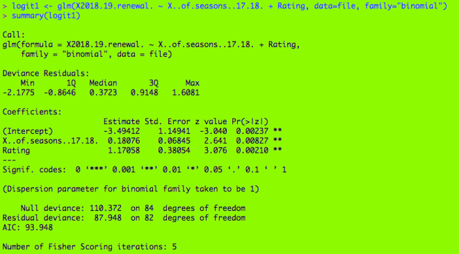
Here’s my first logistic regression model, with my binary variable and two dependent variables (season count and rating). If you’re wondering what the output means, check out R Lesson 4: Logistic Regression Models for a more detailed explanation.

Here are two functions you need to help set up the model. The top function help set up the grid and designate which categorical variable you want to use in your graph. The bottom function helps predict the probabilities of renewal for each show in a certain category. In this case, it would be the rating category (the ones with TV-G, TV-PG, etc.)

Here’s the ggplot function. Geom_line() creates the lines for each level of your categorical variable; here are 5 lines for the 5 categories.

Here’s the graph. As you see, there are five lines, one for each of the ratings. What are some inferences that can be made?

  • The TV-G shows (category 1) usually have the lowest chance of renewal. In this model, a TV-G show would need to have run for approximately a minimum of 22 seasons for at least 50% chance of renewal. (Granted, the only TV-G show on this database is Fixer Upper, which was not renewed)
  • The TV-PG shows have a slightly better chance at renewal as renewal odds for these shows are at least 25%. To attain at a minimum 50% of renewal, these shows would only need to have run for approximately a minimum of 17 seasons, not 22 (like The Simpsons).
  • The TV-14 shows have a minimum 50% chance of renewal, regardless of how many seasons they have run. They would need to have run for at least 25 seasons to attain a minimum 75% chance of renewal, however (SNL would be the only applicable example here, as it was renewed and has run for 43 seasons).
  • The TV-MA shows have a minimum 76% (approximately) chance of renewal no matter how many seasons they have aired. Shows like South Park, Archer, Real Time, Big Mouth and Orange is the New Black are all TV-MA, and all of them were renewed.
  • The unrated shows had the best chances at renewal, as they had a minimum 92% (approximately) chance at renewal. (Granted, Watch What Happens Live! is the only unrated show on this list)

Next, we repeat the process used to create the plot for the first model for these next two models.

What are some inferences that can be made? (I know this graph is hard to read, but we can still make observations from this graph.

  • The orange line (representing Tuesday shows) is the lowest on the graph, so this means Tuesday shows usually had the lowest chances of renewal. This makes sense, as Tuesday shows like LA to Vegas, The Mick, and Rosanne were all cancelled.
  • On the other end, the pink line (representing shows that either aired on streaming services, did not have a consistent time slot, or aired every day like talk shows) is the highest on the graph, so this means shows without a regular time slot had the best chances at renewal (such as Atypical, Jimmy Kimmel Live!, and House of Cards).

What inferences can we make from this graph?

  • The network shows (from the 5 major broadcast networks CBS, ABC, NBC, FOX and the CW) had the lowest chances at renewal. At least 11 seasons would be needed for a minimum 50% chance of renewal.
    • Some shows would include The Simpsons (29 seasons), Family Guy (16 seasons), The Big Bang Theory (11 seasons), and NCIS (15 seasons), all of which were renewed.
  • The cable shows (from channels such as Comedy Central, HBO, and Bravo) have a minimum 58% (approximately) chance of renewal, but at least 15 seasons would be needed for a minimum 70% chance of renewal.
    • Some shows would include South Park (21 seasons) and Real Time (16 seasons), both of which were renewed.
  • The streaming shows (from services such as Netflix, Hulu, or CBS All Access) had the best odds for renewal (approximately 76% minimum chance at renewal). At least 30 seasons would be needed for a 90% chance at renewal.
    • This doesn’t make any sense yet, as streaming shows have only been around since the early-2010s.

Thanks for reading, and I’ll be sure to have the MySQL database ready so you can start learning about querying.

Michael


MySQL Lesson 2: Launching the Database & Inserting Records

Advertisements

Hello everybody,

It’s Michael, and I thought the prefect place to continue from last post would be to show you guys how to launch the database as well as insert records into the database.

But first, I have some corrections to make. This will be the diagram we will use

It’s similar to the one in the previous post, except for one less foreign key in the Awards table that should not have been there along with some other added and modified attributes such as

  • The release year for album has been changed to release date.
  • The featured artist and singer tables have new and/or modified attributes, which include
    • Gender-the gender of the singer/featured artists (it can be null if we are analyzing a group)
      • This is the only addition to the singer table.
    • Age-the age of the featured artist as of August 1, 2018.
    • Birthplace-the birthplace of the featured artist (or where a group was formed)
    • Death-the date of death of the singer/featured artist
      • This was a new column for the featured artist table, but it was on the singer table (I just changed the name from “Date of Death” to Death”)

Now that I got that clarified, the next question would be “How do we launch the database?” We do so with a process called forward engineering (under the database drop-down menu click forward engineering). Forward engineering allows us to export our diagram to an SQL server.

  • You’ll also see an option for reverse engineering in the drop-down menu. You won’t need it to launch the database, but just if you’re wondering what reverse engineering is, it’s essentially the opposite of forward engineering, where you can extract the ER diagram from a launched database (this process can come in handy if you want to modify attributes or relationships in the diagram, but remember to forward engineer again)


Alright, now here’s how to forward engineer your database.

First step is connection options. Choose “new connection” for stored connection and “Standard (TCP/IP)” for connection method. Keep everything else as is.

Next step would be setting up options for the database to be created. Personally, the only two boxes I would check include “Generate INSERT statements for tables” and “Include model attached scripts”.

Next we have to select the objects to forward engineer. Since there are only table objects so far in this diagram, then table objects are the only thing we will be forward engineering. If you’re wondering what the show filter button does, it just allows you to select which tables you don’t want to (or want to) include in the final diagram. Since all five tables are relevant to the database, ignore the show filter column.

If your forward engineering process succeeds, then you will see green checkmarks by each item and the message “Forward Engineer Finished Successfully”.

  • However, if your forward engineering process had errors, then you will be notified. There will be a white box showing you what exactly your error is. This happened to me the first time I tried to forward engineer, as the fields of data type TIME() had 10 as the maximum length while 6 can be the maximum length for fields with data type TIME(). I fixed the error, ran the forward engineering process again, and it worked, as shown below.

Now let’s check to see if our database successfully launched.To do so, click on the schemas tab, then click the loading icon. If you see something called “mydb”, then the database successfully loaded onto the MySQL server.

Now our database is active, but it’s also empty. So, let’s fill it up (and we’re gonna need to fill up all 5 tables separately). So, we use SELECT * FROM mydb.(whatever table you want to insert data into) to first check out the table (the output is shown in the bottom half of the screen). The output, as seen on the bottom half of the picture, shows that the table is empty.

Now let’s add a record to the table and see what happens.

  • Note-this was before I decided to add a gender field. But the procedure is basically the same.

If the “Apply Script Process” is successful, then the next time you run the (SELECT * FROM mydb.Singer) prompt, you should see the record added into the database.

The same procedure applies to fill in other records for this table

  • The process wasn’t successful for me at first, but this was only because my “Date of Death” values should have been formatted like Year-Month-Day, not Month/Day/Year.

Here’s a screenshot of the database with the gender field filled out.

Now let’s fill out the album table (because it connects to the idSinger column)

  • And if you’re wondering what to put for Singer_idSinger, refer back to the Singer table to figure out which primary key in that table corresponds to the album.

And if forward engineering succeeds, then this record should pop up the next time you run (SELECT * FROM mydb.Album).

Let’s add two more records to see what happens.

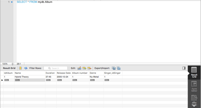
Here’s the output, and in case you’re wondering, I set the idAlbum primary key field to auto-increment, so all I had to do was type 1 as the Hybrid Theory primary key, then the primary keys for the rest of the albums were automatically generated.

If you know how to fill in one table, then you can figure out how to fill out the rest. I’ll actually get into querying with my next post.

Thanks for reading,

Michael

MySQL Lesson 1: Building an ER Diagram

Advertisements

Hello everybody,

This is Michael, and as I mentioned in the last post, I will start building the database that I will be using for this series of posts.

The database will store information about 54 albums (3 for each year from 2000 to 2018) such as track listings, artists, featured artists on certain tracks, genre, release year, duration (of album and individual track), etc.

In the previous post, I did mention that MySQL is meant for query-based analysis. However, before beginning to do queries, we must create our database. As the title explains, this post will focus on the creation of an ER (entity-relationship) diagram. An ER diagram is a graphical representation of items in a database (in this case, albums, track listings, artists, etc.) and how they are related to each other (like how albums can have several track listings).

So, without further hesitation, here is the ER diagram for the database I will be using.

Now you may be confused by all of the arrows and tables in the diagram. Here’s an explanation.

  • This ER diagram will represent the relationship between albums and singers, songs on the album, featured artists, as well as any awards the album either won or received nominations.
  • How do all of these tables relate to each other? Here’s how.
    • Each album must have several tracks, while each track belongs to one and only one album (the thing that looks like a three-pointed arrow means “many” while the thing with two vertical lines represents “one”)
    • Each track can have several, one, or no feature artists (that’s why you see a circle) but each featured artist must belong to one and only track.
    • Each singer can appear more than once (if they have several albums in the database) or just once but each album must correspond to one and only one singer.
    • Each album can be nominated for one or several awards (eg. Grammys, MTV VMAs, etc.) but each award must correspond to only one album.
      • You’ll notice that this is the only dotted line in the diagram. This is because the relationship between album and awards is non-identifying, meaning that you can identify the award based on idAwards field alone, without needing the album field for identification.
      • As for the rest of the relationships (which are known as identifying relationships), each table is dependent on the other table for identification
        • For example, you can’t identify a featured artist without knowing what track they appear on. Likewise, you can’t identify a song without knowing what album it is a part of. Nor can you identify an album without knowing which singer/group created it.

Now what about the attributes in each table (those are the things with diamonds right by them)? Here’s what each of them mean.

  • The album field contains the attributes
    • Name-the name of the album
    • Duration-how long the album is (given in hours:minutes:seconds)
    • Release Year-the year the album came out
    • Album number-how many albums has the artist made up through that point; in other words, is this the artist’s 1st album? 4th? 5th?
    • Genre-the genre of the album
  • The singer field contains the attributes
    • Singer Name-the singer’s (or group’s) name
    • Age-the singer’s age as of August 1, 2018 (if they are still living)
    • Birthplace-the singer’s birthplace (or where the group was formed)
    • Date of Death-the date the artist died
      • You’ll notice the attributes age and date of death have white diamonds right by them; this is because each of them can be null (have no value). For instance, the date of death field can stay blank for living artists. For the other attributes that have blue diamonds besides them, they have to have some sort of value (can’t be null in other words).
  • The tracks field contains the attributes
    • Track Name-the song’s name
    • Track Duration-the length of the song (given in hours:minutes:seconds)
  • The featured artist field contains the attribute
    • Featured artist name-the name of any artist who appears on a particular track
  • The awards field contains the attributes
    • Ceremony-the ceremony where the album either was nominated for or won an award (Grammys, Billboard Music Awards, etc.)
    • Ceremony Year-the year of the ceremony where the album either got nominated for or won an award
    • Won/Nominated-whether an album won or was nominated for a particular award

But wait, what are those keys right by some of the attributes? Those are called primary keys, which are one or more columns with data used to uniquely identify each row in the table. Primary keys are usually stored in auto-incrementing indexes (starting with 1, then 2, then 3, and so on) to ensure uniqueness. For example, in the album table, 1 would be the primary key for the first album in the database, then 2, then 3, all the way to 54.

Take this part of the diagram:


idSinger and idAlbum are both primary keys in their respective tables. But wait, why does Singer_idSinger1 appear in the album table? That is because Singer_idSinger1 is a foreign key, which is a column or set of columns in a table that refers to the primary key in another table-which would be the primary key for the singer table. Foreign keys basically serve as a means to connect the referencing table (album) with the referenced table (singer).

If you want to know how primary keys and foreign keys differ from each other, here’s a handy table (Source-https://www.essentialsql.com/what-is-the-difference-between-a-primary-key-and-a-foreign-key/)

That’s all for now. Thanks for reading,

Michael

What is MySQL?

Advertisements

Hello everybody,

This is Michael, and as I mentioned in the welcome post, I will include other programming languages on this blog. Don’t worry, I’ll still post plenty of R lessons and analyses, but I thought it was time to include other programming languages. The next one I will introduce is MySQL, which is an open-source (meaning free to use) relational database system.

  • Relational databases are created to recognize relations among items in a database. Let’s say you wanted to make a database of NFL teams and include team name, quarterback, running back, center, safety, linebacker, wide receiver, and any other football positions I missed here, along with season record. Team name would be related to any of the positions I just mentioned, as teams have someone for each of the positions. Team name would also be related to season record, as each team has a win-loss-or-sometimes-tie record each year.

To clarify, MySQL and SQL are two totally different things, being that MySQL is database management software whereas SQL is a programming language (it stands for structured query language) used to manage relational databases.

Another thing I wanted to point out is that MySQL and R-although they are both great analytical tools-serve two different purposes. Personally, I would use R to analyze data from a statistical standpoint (as seen by my logistic regression posts) while I would use MySQL for query-based analysis. Each tool has its pros and cons, as R is better for analysis and visualization of data yet the syntax is more complicated than MySQL (that’s just my opinion). Likewise, MySQL is great for query-based analysis, which is more difficult to do in R, but isn’t the best for performing advanced analyses or creating data visualizations. MySQL is also restricted to relational databases, while R is not.

For this series of posts, I’ll build a database (I’ll be using the same database throughout this series of MySQL posts) using MySQL Workbench, which I’d recommend for anyone wanting to make their own MySQL databases. If you want to install it, here’s a handy link-http://www.ccs.neu.edu/home/kathleen/classes/cs3200/MySQLWorkbenchMAC10.pdf

Don’t worry everybody, I’ll actually start building the database with my next MySQL post. This post was just meant to explain the basics of MySQL.

Thank you for reading,

Michael