Python Lesson 26: Cleaning a Pandas Data-frame (pandas pt.3)

Advertisements

Hello everybody,

It’s Michael here, and today’s lesson will be on cleaning a pandas data-frame (pt.3 in my pandas series).

Analyzing data certainly gives you useful insights on your data-however, most real life datasets don’t look as neat as the datasets we’ve worked with over the course of this blog’s run. Oftentimes, real life datasets can be quite messy, which means you’d need to tidy them up before working with them.

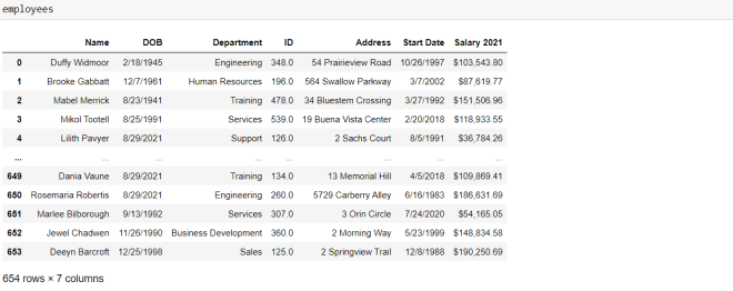
Here’s the messy dataset we’ll be working with in this post:

This datasets contains data regarding 650 employees at a company. And in case you’re wondering, unlike with most of my blog posts, this data doesn’t pertain to anything in real life. I completely made it up.

Now, let’s open up our IDE, import the pandas package, and read our data-frame into our IDE:

import pandas as pd

employees = pd.read_csv('C:/Users/mof39/OneDrive/Documents/Employee data.csv')
  • Keep in mind that the dataset I’m using and the dataset I provided for you guys have different names-that’s because WordPress doesn’t let me upload CSVs and the read_csv function doesn’t work with XLSX files. The dataset I provided for you guys and the dataset I’m using in this code is the same dataset-just named differently so I can easily distinguish between the CSV and XLSX files.

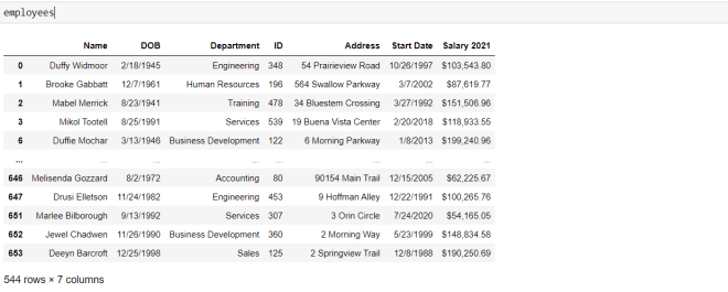
Great! Now, let’s take a look at the head of our data-frame:

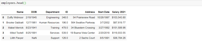
As you can see, our dataset has seven variables. Let’s explore what each variable represents:

  • Name-The name of the employee
  • DOB-The employee’s date of birth
  • Department-The employee’s department in the company
  • ID-The employee’s employee ID number
  • Address-The employee’s home address
  • Start Date-The date the employee started with the company
  • Salary 2021-The employee’s base (pre-tax) salary for the calendar year 2021.

However, we can’t yet create any visualizations with this data or conduct any meaningful analyses. Here are the things we must clean up first:

  • Two employee records are repeated multiple times.
  • There are several null records in the DOB column.
  • Several records in the ID column are stored as float, not int.

First, let’s take care of the null records in the DOB column. When dealing with null/blank records in a data-frame, there are two ways you can deal with this issue:

  • Remove the rows with null values from the dataset.
  • Replace the null values with a specific value or the mean/median/mode of the values in the column.

Well, since the null records are found in a date column, replacing the nulls with the mean/median/mode won’t work here. We could replace the null records in the DOB column with something like 1/1/2021 or we could remove the rows with null records altogether.

In this case, let’s remove the null records altogether. Here’s the code to do so:

employees.dropna(inplace=True)

You will only need a single line of code with the dropna() function in order to drop all null rows from the dataset. Now, you’re probably wondering what inplace=True means-this line of code signifies that you want to drop all null rows from your current data-frame. If you don’t include this line of code, a new data-frame with the null rows removed will be created-your current data-frame (employees) won’t be changed at all.

Now, let’s see what the dataset looks like without the null rows:

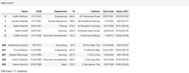
As you can see, there are now 548 rows in the dataset (there were 654 rows before we removed the null records).

But what if you didn’t want to remove all the records with null birthdates? What if you simply wanted to fill all null DOB records with a placeholder date-let’s say 8/29/2021. Here’s the code you’d need to run:

employees["DOB"].fillna("8/29/2021", inplace=True)

To replace all the null values in a certain column with a placeholder value, use the fillna() function with two parameters-the value you’d want to use to replace the null values and the inplace=True line. The inplace=True line works the same way here as it does with the dropna() function.

Another thing to note is that if you only want to replace the null values in a specific column, you’d need to specify that column before the fillna() function. If you don’t do this, ALL null values in the data-frame will be replaced, which isn’t ideal since the values in each column of your data-frame are usually of different data types.

Now, the second bit of cleaning we’d need to do is to change the ID values to type int-they are currently of type float. Here’s the code we’d use to change the data type of values in a pandas data-frame column:

employees["ID"] = pd.to_numeric(employees["ID"], downcast="integer")

To change the data type of the values in the ID column from floats to integers, use the to_numeric() function and pass in two parameters-the column that you want to format (employees["ID"]) in this case and downcast=integer. The reason for the downcast=integer line is to ensure all of the values in the ID column will be converted into integers. Had we not included this line, the data type of the values in the ID column would’ve still been floats.

Now, let’s see what the table looks like after this modification:

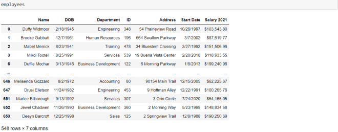
As you can see, all of the values of the ID column are now integers.

  • Note, this is what the data-frame looks like after I dropped the null DOB values, not after I filled the null DOB values with 8/29/2021.

Last but not least, I mentioned that two employees’ records are duplicated. Let’s see how we can remove duplicate values from a data-frame:

employees.drop_duplicates(inplace=True)

To remove the duplicates from the data-frame, simply use the drop_duplicates() function and pass in the parameter inplace=True.

Last but not least, let’s export our cleaned data-frame to a CSV file. Here’s the code to do so:

employees.to_csv('C:/Users/mof39/OneDrive/Documents/Employee data cleaned.csv')

After specifying the data-frame you want to export, use the to_csv() function to export the data-frame. You’ll need to pass in 1 parameter-the location on your computer where you want to store the cleaned data frame. It’s that simple.

Thanks for reading,

Michael

R Lesson 11: Missing Data and Basic K-Means Clustering

Advertisements

Hello everybody,

It’s Michael, and today I will be discussing an unsupervised machine learning technique (recall that from my previous R post?) known as k-means clustering. I will also discuss what to do with missing data observations in a column. I know those may seem like unrelated topics, but the dataset I will be working with utilizes both of those topics.

Here’s the dataset for those who want to work with it-2018 films (1).

But first, as always, let’s load the dataset into R and try to understand our variables:

This dataset contains all 212 wide-release movies for the year 2018. There are seven variables in this dataset:

  • Title-the title of the movie
  • US.Box.Office.Gross-How much money the movie made in the US (this doesn’t factor in worldwide grosses)
    • I got this data from BoxOfficeMojo.com. Great site to collect movie-related data (IMDB works too).
  • Release.Date-The date a movie was released
    • Remember to use the as.Date function seen in the picture to convert your dates from factor type to date type.
  • Genre-The genre of the movie
  • RT.Score-The movie’s critic score on Rotten Tomatoes; 0 represents a score of 0% while 1 represents a score of 100%
  • Audience.Score-The movie’s audience score on Rotten Tomatoes; just as with RT Score, 0 means 0% and 1 means 100%
  • Runtime-The movie’s runtime in minutes; so 100 minutes represents a movie that is 1 hour 40 minute long.

Now, the datasets I’ve used so far have been perfect and tidy. However, real datasets aren’t like that, as they are often messy and contain missing observations, which is the case with this dataset. So what should we do?

First, let me demonstrate a function called missmap that gives you a visual representation of missing observations (and the locations of those observations):

First, before creating the missmap, you need to install the Amelia package and use the library(Amelia) function. Then all you need to do is write missmap(file)-or whatever you named your file-to display the missingness map (that’s why the function is called missmap)

According to this missmap, there aren’t too many missing observations (only 1% as opposed to the 99% of present observations). The few missing observations are located in the RT Score and Audience Score columns, since some of the movies are missing critic or audience scores.

  • Keep in mind that this dataset is only a warmup; I will be working with messier datasets in future posts, so stay tuned.

So how can we tidy up our dataset? Well, here’s one way of approaching it:

na.rm=TRUE

This line of code would be included in my k-means model to tell it to exclude any NA (or missing) data points. I set na.rm to TRUE since TRUE represents any missing data points.

I could also replace all the missing values with the means for RT Score and Audience Score (62% and 66% respectively), but since missing values only make up 1% of all my data, I’ll just stick with excluding missing values.

Now, it’s time to do some k-means clustering. But first of all, what is k-means clustering?

K-means clustering is an unsupervised machine learning algorithm that tries to group data into k amount of clusters by minimizing the distance between individual observations. The aim of k-means clustering is to keep all the data points in a cluster as close to the centroid (center data point) as possible. In order do so, each data point must be assigned to the closest centroid   utilizing Euclidean distance. Euclidean distance is data science lingo for straight line distance between a point in a cluster and the cluster’s centroid.

So the next step in our analysis would be to select the variables to use in our k-means clustering. We can do so by subsetting the data like this:

I chose two columns to include in my subset (US Box Office Gross and RT Score), which creates a data frame that I will use in my k-means clustering. The head function simply displays the first six rows of my subset (the first six box office grosses listed along with their corresponding RT score).

  • For k-means clustering, you should only include two columns in your subset

Now the next step would be to create our clusters. Here’s how:

I first created the movieCluster variable to store my k-means model using the name of my data subset-data1-, the number of clusters I wish to include (5), and nstart (which tells the model to start with 35 random points then select the one with the lowest variation).

  • I didn’t mention it here, but I included the line data1 <- na.omit (data1) in order to omit any rows with NA in them from my subset (remember RT Score had NA values). The k-means model won’t run if you don’t omit NA values (or replace them with means, but for now let’s stick to omitting the values).

I then type in movieCluster to get a better idea of what my cluster looks like. The first thing that is displayed is “K-means clustering with (x) clusters of sizes:”, which shows you  the sizes of each cluster. In this case, the clusters in my k-means model have 62, 22, 3, 10, and 102 observations, respectively. In total, 199 observations were used, which means 13 weren’t used since their RT Scores were missing.

The next thing you see is cluster means, which give you the means of each variable in a certain cluster; in this case, the means for US Box Office Gross and RT Score are displayed for all 5 clusters.

After that, you will see the clustering vector, which will tell you what cluster each observation belongs to (labelled 1-5). As you can see, there are some missing observations (such as 201 and 211); this is because I omitted all NA rows from my data subset (and in turn, my k-means model).

Next you will see the within cluster sum of squares for each cluster; this is a measurement of the variability of the observations in each cluster . Usually the smaller this amount is, the more compact the cluster. As you can see, all of the WCSSBC (my acronym for within cluster sum of squares by cluster) are quite large; this is possibly due to the fact that most of the values in the US Box Office Gross column are over 500,000. I’d probably have smaller WCSSBC if the US Box Office Gross values were smaller, but that’s neither here nor there.

The last thing you will see is between_SS/total_SS=95.4%, which represents the between sum-of-squares and total sum-of-squares ratio; this is a measure of the goodness-of-fit of the model. 95.4% indicates that there is an excellent goodness-of-fit for this model.

Last but not least, let’s graph our model. Here’s how:

The movies are clustered by US Box Office Gross (referred here as simply Box Office Gross); the colors of the dots represent each cluster. Here’s what each color represents:

  • Light blue-movies that made between $0 to $25 million
  • Black-movies that made between $25 to $100 million (many limited releases)
  • Red-movies that made between $100 to $200 million
  • Dark blue-movies that made between $200 to $400 million
  • Green-movies that made between $600 to $700 million

As you can see, the green cluster is the outlier among the data, since only 3 movies in our dataset made at least $600 million (Black Panther, Avengers Infinity War, and Incredibles 2).

Thanks for reading,

Michael