Python Lesson 37: Intro to Neural Networks (AI pt. 1)

Advertisements

Hello everybody,

Michael here, and for today’s post, I’ll discuss something a little different-neural networks; this is the first post of my new AI (artificial intelligence) series. Granted, I’ll be using Python, which I’ve used quite a bit in this blog (this is my 37th Python lesson after all).

More specifically, in today’s post, I will be discussing the basics of neural networks and how to set up a simple neural network in Python. And in case you’re wondering (and/or really enjoy AI content), the remainder of my 2022 blog posts AND my first few 2023 posts will cover neural networks.

But first, a little bit about machine learning…

For those of you who’ve been following my blog for quite a while, you may recall that a lot of my earlier entries covered machine learning.

But what is machine learning exactly? It’s essentially a process where you are training a program to do something (like identifying a certain plant from a photo)-or in better terms, training a machine to learn something (hence the term machine learning). One of my early posts from February 2019-R Lesson 10: Intro to Machine Learning-Supervised and Unsupervised-does a good job of explaining some of the basics of machine learning. Granted, I wrote this post as part of a series of R lessons, but the gist of the post can be applied to any programming/automation tool.

Now onto neural networks

What is a neural network (in the context of programming)? To help explain this concept, think of the way all of the neurons in your brain process information. Neural networks operate in a similar manner, as they are meant to process information via a computer program that’s meant to mimic the way our brains process information.

Neural networks are a form of machine learning, and just like machine learning, you can utilize supervised and unsupervised machine learning with neural networks. Unsupervised machine learning with neural networks actually has a name of its own-deep learning, which is a process you use to allow the neural network to train itself rather than coding in any guidance for the neural network’s operation.

A neural network you’ve likely come across

A neural network you’ve most likely seen or heard of before is deepfakes. If you’ve ever seen a video where it appears someone’s face looks stitched onto someone else’s body-that’s deepfake AI at work.

A great example of deepfake AI at work was seen on season 17 (2022) of America’s Got Talenthttps://www.youtube.com/watch?v=Jr8yEgu7sHU&t=116s. The act in the linked video-Metaphysic-utilized deepfake AI to make it appear as if the king of rock’n’roll Elvis and judges Sofia Vergara and Heidi Klum were singing Elvis’s greatest hits. Take a closer look at the video, and you realize that “Elvis”, “Sofia”, and “Heidi” are being animated by three singers in real-time standing in front of projectors. Pretty neat stuff, right? Plus, Metaphysic finished the season in 4th place-not too shabby for AGT’s first deepfake/metaverse AI act.

Another brilliant, albeit controversial, example of deepfake AI at work can be found in Kendrick Lamar’s 2022 music video for The Heart Part 5https://www.youtube.com/watch?v=uAPUkgeiFVY (highly recommend listening to Mr. Morale & the Big Steppers). In this video, Kendrick Lamar uses deepfake AI to transform himself into six notable celebrities-OJ Simpson, Kanye West, Jussie Smollett, Will Smith, Kobe Bryant, and Nipsey Hussle-while rapping six different verses from the perspectives of these individuals.

Did I cover neural networks before?

Did I ever explicitly cover neural networks before? No.

However, several past posts did cover machine learning-both supervised and unsupervised. Here are a few of those posts:

Thanks for reading,

Michael

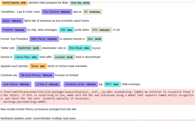
Python Lesson 36: Named Entity Recognition (NLP pt. 5)

Advertisements

Hello everybody,

Michael here, and today’s lesson will be on named entity recoginition in Python NLP.

Intro to named entity recognition

What is named entity recogintion exactly? Well, it’s NLP’s process of identifying named entities in text. Named entities are bascially anything that is a place, person, organization, time, object, or geographic entity-in other words, anything that can be denoted with a proper name.

Take a look at this headline from ABC News from July 21, 2022:

Former Minneapolis police officer sentenced in George Floyd killing

How many named entities can you find? If you answered two, you’d be correct-Minneapolis and George Floyd.

Python’s SPACY package

Before we begin any named-entity recognition analysis, we must first pip install the spacy package using this line of code-pip install spacy. Unlike the last four NLP lessons I’ve posted, this lesson won’t use the NLTK package (or any modules within) as Python’s spacy package is better suited for this task.

In case you need assistance with installing the spacy package, click on this link-https://spacy.io/usage#installation. This link will show you how to install spacy based on what operating system you have.

If you go to this link, you will see an interface like the one pictured above (picture current as of July 2022). Toggling the filters on this interface will show you the commands you’ll need to use to install not only the spacy module itself but also a trained spacy pipeline in whatever language you choose (and there are 23 options for languages here). The commands needed to install spacy will depend on things like the OS you’re using (whether Mac, Windows, or Linux), the package manage you’re using to install Python packages (whether pip, conda, or from source), among other things.

The Spacy pipeline

Similar to how we downloaded the punkt and stopwords modules in NTLK, we will also need to install a seprate module to work with spacy-in this case, the spacy pipeline. See, to ensure the spacy package works to its fullest capabilites, you’ll need to download a spacy pipeline in whatever language you choose (I’m using English for this example)

  • Remember to install the spacy pipeline AFTER installing the spacy package!

For this lesson, I’ll be using the en_core_web_md pipeline, which is a medium-sized English spacy pipeline. If you wish, you can download the en_core_web_sm or en_core_web_lg pipelines-these are the small-sized and large-sized English spacy pipelines, respectively. The larger the spacy pipeline you choose, the better its named-entity recognition functionalities would be-the small pipeline has 12 megabytes of info, the medium pipeline has 40 megabytes of info, and the large pipeline has 560 megabytes of info.

To install the medium-sized English spacy pipeline, run this command-python -m spacy download en_core_web_md.

  • If you’re downloading the small-sized or large-sized English spacy pipelines, replace en_core_web_md with en_core_web_sm or en_core_web_lg depending on the pipeline size you’re using.

However, even after installing the pipeline, you’ll still need to download it in your code using this line of code-spacy.load('en_core_web_md'). Remember that even though I’m using the en_core_web_md spacy pipeline, pass whatever pipeline you’ll be using as the parameter for the spacy.load() method.

Spacy in action

Now that I’ve explained the basics of setting up spacy, it’s time to show named-entity recognition in action. For the example I’ll show you, I’ll use this XLSX file containing twelve different news headlines from the Associated Press published on July 25 and 26, 2022:

Let’s see how we can find all of the named entities in these twelve headlines:

import spacy
nlp = spacy.load('en_core_web_md')
import pandas as pd

headlines = pd.read_excel(r'C:\Users\mof39\OneDrive\Documents\headlines.xlsx')

for h in headlines['Headline']:
    doc = nlp(h)
    
    for ent in doc.ents:
        print(ent.text)
    
    print(h)
    print() 

North Dakota
final day
North Dakota abortion clinic prepares for likely final day

Paul Sorvino
83
‘Goodfellas,’ ‘Law & Order’ actor Paul Sorvino dies at 83

Biden
Biden fights talk of recession as key economic report looms

Hobbled
GM
40%
Hobbled by chip, other shortages, GM profit slides 40% in Q2

Mike Pence
Nov.
Former Vice President Mike Pence to release memoir in Nov.

September
Elon Musk
Twitter sets September shareholder vote on Elon Musk buyout

Choco Taco
summer
Sorrow in Choco Taco town after summer treat is discontinued

Texas
Appeals court upholds Texas block on school mask mandates

QB Kyler Murray
Cardinals say QB Kyler Murray focused on football

Jack Harlow
Lil Nas X
Kendrick Lamar
MTV
Jack Harlow, Lil Nas X, Kendrick Lamar top MTV VMA nominees

New studies bolster theory coronavirus emerged from the wild

Northwest swelters under ‘uncomfortable’ multiday heat wave

In this example, I first performed all the necessary imports and read in the headlines dataset as a pandas dataframe. I then looped through all the values in the Headline column in the pandas dataframe, converted each value into a spacy doc (this is necessary for the named-entity recognition), and looped through all the tokens in the headline in order to find and print out any named entities that spacy finds-the headline itself is printed below all (or no) named entities that are found.

As you can see, spacy found named entities in 10 of the 12 headlines. However, you may notice that spacy’s named-entity recognition isn’t completely accurate, as it missed some tokens that are clearly named entities. Here are some surprising omissions:

  • Goodfellas and Law & Order on headline #2-referring to a movie and TV show, respectively
  • Q2 on headline #4-in the context of this article, refers to GM’s Q2 2022 profits
  • Twitter on headline #6-Twitter is one of the world’s most popular social media sites after all
  • Cardinals on headline #9-This headline refers to Arizona Cardinals QB Kyler Murray
  • VMA on headline #10-VMA refers to the MTV VMAs, or Video Music Awards
  • Northwest on headline #12-Northwest referring to the Northwest US region

Along with these surprising omissions, here are some other interesting observations I found:

  • Spacy read QB Kyler Murray as a single entity but not Vice President Mike Pence
  • MTV VMA wasn’t read as a single entity-rather, MTV was read as the entity
  • Hobbled shouldn’t be read as an entity at all

Now, what if you wanted to know each entity’s label? Take a look at the code below, paying attention to the red highlighted line (the line I revised from the above example):

import spacy
nlp = spacy.load('en_core_web_md')
import pandas as pd

headlines = pd.read_excel(r'C:\Users\mof39\OneDrive\Documents\headlines.xlsx')

for h in headlines['Headline']:
    doc = nlp(h)
    
    for ent in doc.ents:
        print(ent.text + ' --> ' + ent.label_)
    
    print(h)
    print() 

North Dakota --> GPE
final day --> DATE
North Dakota abortion clinic prepares for likely final day

Paul Sorvino --> PERSON
83 --> CARDINAL
‘Goodfellas,’ ‘Law & Order’ actor Paul Sorvino dies at 83

Biden --> PERSON
Biden fights talk of recession as key economic report looms

Hobbled --> PERSON
GM --> ORG
40% --> PERCENT
Hobbled by chip, other shortages, GM profit slides 40% in Q2

Mike Pence --> PERSON
Nov. --> DATE
Former Vice President Mike Pence to release memoir in Nov.

September --> DATE
Elon Musk --> ORG
Twitter sets September shareholder vote on Elon Musk buyout

Choco Taco --> ORG
summer --> DATE
Sorrow in Choco Taco town after summer treat is discontinued

Texas --> GPE
Appeals court upholds Texas block on school mask mandates

QB Kyler Murray --> PERSON
Cardinals say QB Kyler Murray focused on football

Jack Harlow --> PERSON
Lil Nas X --> PERSON
Kendrick Lamar --> PERSON
MTV --> ORG
Jack Harlow, Lil Nas X, Kendrick Lamar top MTV VMA nominees

New studies bolster theory coronavirus emerged from the wild

Northwest swelters under ‘uncomfortable’ multiday heat wave

To print out each entity’s label, I added a text arrow after each entity pointing to that entity’s label. What do each of the entity labels mean?

  • ORG-any sort of organization (like a company, educational institution, etc)
  • NORP-nationality/religious or political groups (e.g. American, Catholic, Democrat)
  • GPE-geographical entity
  • PERSON
  • LANGUAGE
  • MONEY
  • DATE
  • TIME
  • PRODUCT
  • EVENT
  • CARDINAL-as in cardinal number (one, two, three, etc.)
  • ORDINAL-as in ordinal number (first, second, third, etc.)
  • WORK OF ART-a book, movie, song; really anything that you can consider a work of art

All in all, the label matching seems to be pretty accurate. However, one mislabelled entity can be found on headline #6-Elon Musk is mislabelled as ORG (or organization) when he clearly isn’t an ORG. Another mislabelled entity is Hobbled-it is listed as a PERSON when it shouldn’t be listed as an entity at all.

Now, what if you wanted a neat way to visualize named-entity recognition? Well, Spacy’s Displacy module would be the answer for you. See, the Displacy module will help you visualize the NER (named-entity recognition) that Spacy conducts.

Let’s take a look at Displacy in action:

import spacy
nlp = spacy.load('en_core_web_md')
import pandas as pd

headlines = pd.read_excel(r'C:\Users\mof39\OneDrive\Documents\headlines.xlsx')

for h in headlines['Headline']:
    doc = nlp(h)
    displacy.render(doc, style='ent')

Pay attention to the code that I used here. Unlike the previous examples, I actually save the spacy pipeline I downloaded as a variable (nlp). I then read in the data-frame containing the headlines, loop through each value in the Headline column, and run the displacy.render() method, passing in the string I’m parsing (doc) and the displacy style I want to use (ent) as this method’s parameters.

After running the code, you can see a nice, colorful output showing you all the named entities (at least the named entities spacy found) in the text along with the entitiy’s corresponding label. You’ll also notice that each entity is color-coded according to its label; for instance, geographical entites (e.g. Texas, North Dakota) are colored in orange while peoples’ names (e.g. Kendrick Lamar, Lil Nas X) are colored in purple.

While running this code, you’ll also see the UserWarning above-in this case, don’t worry, as this warning simply means that spacy couldn’t find any named entities for a particular string (in this example, spacy couldn’t find any named entities for two of the 12 strings).

Oh, and one more reminder. In the displacy.render() method, you’ll need to include style='ent' as a parameter if you want to work with named-entity recognition, as here’s the default diagram that you get as an output if you don’t specify a style:

In this case, the code still works fine, but you’ll get a dependency parse diagram, which shows you how words in a string are syntactically related to each other.

Thanks for reading,

Michael

Python Lesson 35: Parts-of-speech tagging (NLP pt. 4)

Advertisements

Hello everybody,

Michael here, and today’s post will cover parts-of-speech tagging as it relates to Python NLP (this is part 4 in my NLP Python series).

Intro to parts-of-speech tagging

What is parts-of-speech (POS) tagging, exactly? See, Python NLP can do some really cool things, such as getting the roots of words (Python Lesson 34: Stemming and Lemmatization (NLP pt. 3)) and finding commonly used words (stopwords) in 24 different languages (Python Lesson 33: Stopwords (NLP pt.2)). In Python, parts-of-speech tagging is a quite self-explanatory process, as it involves tokenizing a string and identifying each token’s part-of-speech (such as a noun, verb, etc.). Keep in mind that this isn’t going to be a grammar lesson, so I’m not going to teach you how to use POS tagging to improve your grammar or proofread something you wrote.

POS tagging in action

Now that I’ve explained the basics of POS tagging, let’s see it in action! Take a look at the example below:

import nltk
nltk.download('punkt')
nltk.download('averaged_perceptron_tagger')

test = input('Please input a test string: ')
tokens = nltk.word_tokenize(test)

tagged = []

for t in tokens:
    tagged = nltk.pos_tag(tokens)
    
print(tagged)

Please input a test string: I had a fun time dancing last night.
[('I', 'PRP'), ('had', 'VBD'), ('a', 'DT'), ('fun', 'JJ'), ('time', 'NN'), ('dancing', 'VBG'), ('last', 'JJ'), ('night', 'NN'), ('.', '.')]

Before getting into the fun POS tagging, you’d first need to import the nltk package and download two of the package’s modules-punkt and averaged_perceptron_tagger. punkt is NLTK’s standard package module which allows Python to work its NLP magic while averaged_perceptron_tagger is the module that enables all the fun POS tagging capabilities.

After including all the necessary imports and downloading all the necessary package modules, I then inputted and word-tokenized a test string. I then created an empty list-tagged-that will store the results of our POS tagging.

To perform the POS tagging, I iterated through each element in the list of tokens (aptly called tokens) and used NLTK’s pos_tag() method to add the appropriate POS tag to the element. I then printed out the tagged list, which contains the results of our POS tagging. As you can see, the tagged list contains a list of tuples-the first element in each tuple is the token itself while the second element is that token’s part-of-speech. Punctuation is also included, as punctuation counts as its own token, but doesn’t belong to any part-of-speech.

You likely noticed that the POS tags are all two or three character abbrevations. Here’s a table explaining all of the POS tags:

TagPart-of-speechExample/Explanation
CCcoordinating conjuctionAny of the FANBOYS conjuctions (for, and,
nor, but, or, yet, so)
CDcardinal digitThe numbers 0-9
DTdeterminerA word in front of a noun to specify quanity
or to clarify what the noun refers to (e.g. one
car, that child)
EXexistential thereThere is a snake in the grass.
FWforeign wordSince I’m using English for this post, any word
that isn’t English (e.g. palabra in Spanish)
INprepositionon, in, at
JJadjective (base form)large, tiny
JJRcomparative adjectivelarger, tinier
JJSsuperlative adjectivelargest, tiniest
LSlist marker1), 2)
MDmodal verbOtherwise known as auxiliary verb (e.g. might
happen, must visit)
NNsingular nouncar, tree, cat, etc.
NNSplural nouncars, trees, cats, etc.
NNPsingular proper nounFord
NNPSplural proper nounAmericans
PDTpredeterminerA word or phrase that occurs before a determiner
that quantifies a noun phrase (e.g. lots of toys,
few students)
POSpossessive endingMichael’s, Tommy’s
PRPpersonal pronounPronouns associated with a grammatical person-be it first person, second person, or third person (e.g.
they, he, she)
PRP$possessive pronounPronouns that indicate possession (e.g. mine, theirs, hers)
RBadverbvery, extremely
RBRcomparative adverbearlier, worse
RBSsuperlative adverbbest, worst
RPparticleAny word that doesn’t fall within the main parts-of-speech (e.g. give up)
TOthe word ‘to’to come home
UHinterjectionYikes! Ummmm.
VBbase form of verbwalk
VBDpast tense of verbwalked
VBGgerund form of verbwalking
VBNpast participle of verbwalked
VBPpresent singular form of verb (non-3rd person)walk
VBZpresent singular form
of verb (3rd-person)
walks
WDT“wh” determinerwhich
WP“wh” pronounwho, what
WP$possessive “wh” pronounwhose
WRB“wh” adverbwhere, when

As you can see, even though English has only eight parts of speech (verbs, nouns, adjectives, adverbs, pronouns, prepositions, conjuctions, and interjections), Python has 35 (!) parts-of-speech tags.

  • Even though I’m working with English here, I imagine these POS tags can work for any language.

If you take a look at the last line of output in the above example (the line containing the list of tuples), you can see two-element tuples containing the token itself as the first element along with the token’s POS tag as the second element. And yes, punctuation in a sentence counts as a token itself, but it has no POS tag. Hence why the tuple-POS tag pair for the period at the end of the sentence looks like this-['.', '.'].

Now, what if there was a sentence that had the same word twice but used as different parts-of-speech (e.g. a sentence that had the same word used as a noun and a verb). Let’s take a look at the example below:

import nltk
nltk.download('punkt')
nltk.download('averaged_perceptron_tagger')

test = input('Please input a test string: ')
tokens = nltk.word_tokenize(test)
tagged = nltk.pos_tag(tokens)
    
print(tagged)

Please input a test string: She got a call at work telling her to call the project manager.
[('She', 'PRP'), ('got', 'VBD'), ('a', 'DT'), ('call', 'NN'), ('at', 'IN'), ('work', 'NN'), ('telling', 'VBG'), ('her', 'PRP'), ('to', 'TO'), ('call', 'VB'), ('the', 'DT'), ('project', 'NN'), ('manager', 'NN'), ('.', '.')]

Take a close look at the sentence I used in this example-She got a call at work telling her to call the project manager. Notice the repeated word here-call. In this example, call is used as both a noun (She got a call at work) and a verb (to call the project manager.). The neat thing here is that NLTK’s POS tagger recognizes that the word call is used as two different parts-of-speech in that sentence.

However, the POS tagger may not always be so accurate when it comes to recognizing the same word used as a different part of speech. Take a look at this example:

import nltk
nltk.download('punkt')
nltk.download('averaged_perceptron_tagger')

test = input('Please input a test string: ')
tokens = nltk.word_tokenize(test)
tagged = nltk.pos_tag(tokens)
    
print(tagged)

Please input a test string: My apartment building is bigger than any other apartment in a 5-block vicinity.
[('My', 'PRP$'), ('apartment', 'NN'), ('building', 'NN'), ('is', 'VBZ'), ('bigger', 'JJR'), ('than', 'IN'), ('any', 'DT'), ('other', 'JJ'), ('apartment', 'NN'), ('in', 'IN'), ('a', 'DT'), ('5-block', 'JJ'), ('vicinity', 'NN'), ('.', '.')]

In this example, I’m using the word apartment twice, as both an adjective (My apartment building) and a noun (any other apartment). However, NLTK’s POS tagger doesn’t recognize that the first instance of the word apartment is being used as an adjective to modify the noun building.

  • Hey, what can you say, programs aren’t always perfect. But I’d say NLTK’s POS tagger works quite well for parts-of-speech analysis.

Thanks for reading,

Michael

Python Lesson 34: Stemming and Lemmatization (NLP pt. 3)

Advertisements

Hello everybody,

Michael here, and today’s lesson will cover stemming and lemmatization in Python NLP (natural language processing).

Stemming

Now that we’ve covered some basic tokenization concepts (like tokenization itself and filtering out stopwords), we can move on to the next important concepts in NLP-stemming and lemmatization. Stemming is an NLP task that involves reducing words to their roots-for instance, stemming the words “liked” and “likely” would result in “like”

Now, the NLTK package has several stemmers you can use, but for this lesson (along with all Python NLP lesson on this blog) I will be using NLTK’s PorterStemmer stemmer. Let’s see stemming in action:

import nltk
nltk.download('punkt')
from nltk.stem import PorterStemmer

test = input('Please input a test string: ')
testWords = nltk.word_tokenize(test)
print(testWords)

stemmer = PorterStemmer()
stemmedWords = [stemmer.stem(word) for word in testWords]
print(stemmedWords)

Please input a test string: Byte sized programming classes for eager coding learners
['Byte', 'sized', 'programming', 'classes', 'for', 'eager', 'coding', 'learners']
['byte', 'size', 'program', 'class', 'for', 'eager', 'code', 'learner']

To start your stemming, include the first three lines of code you see above as the imports and downloads. And yes, you’ll need to import the PorterStemmer separately.

After including all the necessary downloads and imports, I then included code to input a test string, word-tokenize that test string, and print the list of tokens. After performing the word-tokenizing, I then created a PorterStemmer object (aptly named stemmer), performed a list comprehension to stem each token in the input string, and printed the stemmed list of tokens.

What do you notice in the stemmed list of tokens (it’s the last line of output by the way)? First of all, all words are displayed in lowercase, which is nothing remarkable. Secondly, notice how most of the stemmed tokens make perfect sense (e.g. sized = size, programming = program, and so on); sometimes when stemming words in Python NLP, you’ll get some weird outputs.

Now, let’s try another input string and see what kind of results we get:

import nltk
nltk.download('punkt')
from nltk.stem import PorterStemmer

test = input('Please input a test string: ')
testWords = nltk.word_tokenize(test)
print(testWords)

stemmer = PorterStemmer()
stemmedWords = [stemmer.stem(word) for word in testWords]
print(stemmedWords)

Please input a test string: The quick brown fox jumped over the lazy brown dog and jumps over the even lazier brown cat.
['The', 'quick', 'brown', 'fox', 'jumped', 'over', 'the', 'lazy', 'brown', 'dog', 'and', 'jumps', 'over', 'the', 'even', 'lazier', 'brown', 'cat', '.']
['the', 'quick', 'brown', 'fox', 'jump', 'over', 'the', 'lazi', 'brown', 'dog', 'and', 'jump', 'over', 'the', 'even', 'lazier', 'brown', 'cat', '.']

Just like the previous example, this example tokenizes an input string and stems each element in the tokenized list. However, pay attention to the words “lazy” and “lazier”. Although “lazier” is a conjugation of “lazy”, “lazy” has a stem of, “lazi” while “lazier” has a stem of “lazier”.

OK, so if stemming sometimes gives you weird and inconsistent results (like in the example above), there’s a reason for that. See, stemming reduces words to their core meaning. However, unlike lemmatization (which I’ll discuss next), stemming is a lot cruder, so it’s not uncommon to get fragments of words when stemming. Plus, the PorterStemmer tool is based off an algorithm that was developed in 1979-so yea, it’s a little dated. There is a PorterStemmer2 tool that improves upon the PorterStemmer tool we used-just FYI.

Lemmatization

Now that we’ve covered the basics of word stemming, let’s move on to word lemmatization. Lemmatization, like stemming, is an NLP tool that is meant to reduce words to their core meaning. However, unlike stemming, lemmatization usually gives you a complete word rather than a fragment of a word (e.g. “lazi” from the previous example).

import nltk
nltk.download('punkt')
nltk.download('wordnet')
from nltk.stem import WordNetLemmatizer

test = input('Please input a test string: ')
tokens = nltk.word_tokenize(test)
lemmatizer = WordNetLemmatizer()
lemmatizedList = [lemmatizer.lemmatize(word) for word in tokens]

print(lemmatizedList)

Please input a test string: The two friends drove their nice blue cars across the Florida coast.
['The', 'two', 'friend', 'drove', 'their', 'nice', 'blue', 'car', 'across', 'the', 'Florida', 'coast', '.']

So, how did I accomplish the lemmatization? First of all, after adding in all the necessary downloads and imports (and typing in an import string), I first tokenized my input string. I then created a lemmatizer object (aptly named lemmatizer) using NLTK’s WordNetLemmatizer tool. To lemmatize each token in the input string, I ran list comprehension to pass each element of the list of tokens (aptly named tokens) into the lemmatizer tool to lemmatize each word. I stored the results of this list comprehension into the lemmatizedList and printed that list below the text input.

As you can see from the example above, the lemmas of the tokens above are the same as the tokens themselves (e.g. two, across, blue). However, some of the tokens have different lemmas (e.g. cars–>car, friends–>friend). That’s because, as I mentioned earlier, lemmas find the root of a word. In the case of the words cars and friends, the root of the word would be the word’s singular form (car and friend, respectively).

  • Just thought I’d put this out here, but the root word that is generated is called a lemma, and the group of words with a particular lemma is called a lexeme. For instance, the word “try” would be the lemma while the words “trying, tried, tries” could be part of (but not the only words) that are part of the lexeme.

So, from the example above, looks like the lemmatization works much better than stemming when it comes to finding the root of a word. But what if you tried lemmatizing a word that looked very different from its lemma? Let’s see an example of that below (using the lemmatizer object created from the previous example):

lemmatizer.lemmatize("bought")
'bought'

In this example, I’m trying to lemmatize the word “bought” (as in, I bought a new watch.) However, you can see that in this example, the lemma of bought is bought. That can’t be right, can it?

Why do you think that particular output was generated? Simply put, the lemmatizer tool, by default, will assume a word is a noun (even when that clearly isn’t the case).

How can we correct this? Take a look at the example below:

lemmatizer.lemmatize("bought", pos='v')
'buy'

In this example, I added the pos parameter, which specifies a part of speech for a particular word. In this case, I set the value of pos to v, as the word “bought” is a verb. Once I added the pos parameter, I was able to get the correct lemma for the word “bought”-“buy”.

  • When working with lemmatization, you’ll run into the issue quite a bit with adjectives and irregular verbs.

Thanks for reading,

Michael

Python Lesson 33: Stopwords (NLP pt.2)

Advertisements

Hello everybody,

Michael here, and today’s post will be on stopwords in Python NLP-part 2 in my NLP series.

What are stopwords? Simply put, stopwords are words you want to ignore when tokenizing a string. Oftentimes, stopwords are common English words like “a”, “the”, and “is” that are so commonly used in English that they don’t add much meaning in text.

  • Stopwords can be found for any language, but for this series of NLP lessons, I’ll focus on English words.

Now that I’ve explained the basics of stopwords, let’s see them in action:

import nltk
nltk.download('punkt')
nltk.download('stopwords')
from nltk.corpus import stopwords

test = input('Please type in a string: ')
testWords = nltk.word_tokenize(test)

stopwordsList = set(stopwords.words('english'))

filteredList = []

for t in testWords:
    if t.casefold() not in stopwordsList:
        filteredList.append(t)

print(filteredList)

Please type in a string: The puppies and the kitties played in their playpen on the hot summer afternoon.
['puppies', 'kitties', 'played', 'playpen', 'hot', 'summer', 'afternoon', '.']

To utilize NLTK’s stopwords module, you’ll need to run the nltk.download(stopwords) command and import the stopwords module from the nltk.corpus package.

  • Yes, you’ll still need to download the punkt module, as it will enable easy tokenization, which is important to have when working with stopwords.

To store the list of tokens in the string you input, create a testWords variable that stores the output of the nltk.word_tokenize function. To get a list of NLTK’s English stopwords, use the line of code set(stopwords.words('english'))-this line of code creates a set from the list of NLTK’s English stopwords. Recall that sets are like lists, except without duplicate elements.

To gather a list of stopwords in the input string, you’d need to first create an empty list-filteredList in this case-that you’ll need to filter the stopwords out of the list of tokens (testWords in this case). To remove the stopwords, you’ll need to iterate through the list of tokens (again, testWords in this case), check if each token is in the list of stopwords and if not, add the token to the empty list you created earlier (filteredList in this case).

As you can see in the example above, the input string I used has 15 tokens (the punctuation at the end of the sentence counts as a token). After filtering out the stopwords, the resulting list only contains 8 tokens, as 7 tokens have been filtered out-The and the in their on the. Yes, even though I am iterating though a UNIQUE list of stopwords, the loop I am running will check for all instances of a stopword and exclude them from the filtered list (after all, there were three instances of the word “the” in the input string).

Ever want to see all of the words included in NLTK’s English stopwords list? Run the command print(stopwords.words('english') and you’ll see all the stopwords NLTK uses in English:

['i', 'me', 'my', 'myself', 'we', 'our', 'ours', 'ourselves', 'you', "you're", "you've", "you'll", "you'd", 'your', 'yours', 'yourself', 'yourselves', 'he', 'him', 'his', 'himself', 'she', "she's", 'her', 'hers', 'herself', 'it', "it's", 'its', 'itself', 'they', 'them', 'their', 'theirs', 'themselves', 'what', 'which', 'who', 'whom', 'this', 'that', "that'll", 'these', 'those', 'am', 'is', 'are', 'was', 'were', 'be', 'been', 'being', 'have', 'has', 'had', 'having', 'do', 'does', 'did', 'doing', 'a', 'an', 'the', 'and', 'but', 'if', 'or', 'because', 'as', 'until', 'while', 'of', 'at', 'by', 'for', 'with', 'about', 'against', 'between', 'into', 'through', 'during', 'before', 'after', 'above', 'below', 'to', 'from', 'up', 'down', 'in', 'out', 'on', 'off', 'over', 'under', 'again', 'further', 'then', 'once', 'here', 'there', 'when', 'where', 'why', 'how', 'all', 'any', 'both', 'each', 'few', 'more', 'most', 'other', 'some', 'such', 'no', 'nor', 'not', 'only', 'own', 'same', 'so', 'than', 'too', 'very', 's', 't', 'can', 'will', 'just', 'don', "don't", 'should', "should've", 'now', 'd', 'll', 'm', 'o', 're', 've', 'y', 'ain', 'aren', "aren't", 'couldn', "couldn't", 'didn', "didn't", 'doesn', "doesn't", 'hadn', "hadn't", 'hasn', "hasn't", 'haven', "haven't", 'isn', "isn't", 'ma', 'mightn', "mightn't", 'mustn', "mustn't", 'needn', "needn't", 'shan', "shan't", 'shouldn', "shouldn't", 'wasn', "wasn't", 'weren', "weren't", 'won', "won't", 'wouldn', "wouldn't"]

In total, NLTK has 179 stopwords in English, which consist of common English pronouns (I, my, you), commonly used English contracations (don’t, isn’t), conjungations of common English verbs (such as be and have), and surprisingly, contractions that you don’t hear most people use nowadays (be honest, when was the last time you heard someone use a word like shan’t or mightn’t).

  • Of course, you can always append words to NLTK’s stopwords list as you see fit, but when working with stopwords in English (or any language), I’d suggest sticking with the default stopwords list.

Now, I know I mentioned that I’ll mostly be working with English throughout my NLP lessons, but let’s explore stopwords in other languages. For this example, I’ll use the same code and same input string I used in the previous example, except this time use Spanish:

Please type in a string: Los cachorros y los gatitos jugaban en su corralito en la calurosa tarde de verano.
['cachorros', 'gatitos', 'jugaban', 'corralito', 'calurosa', 'tarde', 'verano', '.']

So, the Spanish-translated version of my previous example has 16 tokens, 8 of which appear on the filtered list. Thus, there were 8 stopwords that were removed from the testWords list.

Want to see the Spanish list of stopwords? Run the command print(stopwords.words('spanish') and take a look:

['de', 'la', 'que', 'el', 'en', 'y', 'a', 'los', 'del', 'se', 'las', 'por', 'un', 'para', 'con', 'no', 'una', 'su', 'al', 'lo', 'como', 'más', 'pero', 'sus', 'le', 'ya', 'o', 'este', 'sí', 'porque', 'esta', 'entre', 'cuando', 'muy', 'sin', 'sobre', 'también', 'me', 'hasta', 'hay', 'donde', 'quien', 'desde', 'todo', 'nos', 'durante', 'todos', 'uno', 'les', 'ni', 'contra', 'otros', 'ese', 'eso', 'ante', 'ellos', 'e', 'esto', 'mí', 'antes', 'algunos', 'qué', 'unos', 'yo', 'otro', 'otras', 'otra', 'él', 'tanto', 'esa', 'estos', 'mucho', 'quienes', 'nada', 'muchos', 'cual', 'poco', 'ella', 'estar', 'estas', 'algunas', 'algo', 'nosotros', 'mi', 'mis', 'tú', 'te', 'ti', 'tu', 'tus', 'ellas', 'nosotras', 'vosotros', 'vosotras', 'os', 'mío', 'mía', 'míos', 'mías', 'tuyo', 'tuya', 'tuyos', 'tuyas', 'suyo', 'suya', 'suyos', 'suyas', 'nuestro', 'nuestra', 'nuestros', 'nuestras', 'vuestro', 'vuestra', 'vuestros', 'vuestras', 'esos', 'esas', 'estoy', 'estás', 'está', 'estamos', 'estáis', 'están', 'esté', 'estés', 'estemos', 'estéis', 'estén', 'estaré', 'estarás', 'estará', 'estaremos', 'estaréis', 'estarán', 'estaría', 'estarías', 'estaríamos', 'estaríais', 'estarían', 'estaba', 'estabas', 'estábamos', 'estabais', 'estaban', 'estuve', 'estuviste', 'estuvo', 'estuvimos', 'estuvisteis', 'estuvieron', 'estuviera', 'estuvieras', 'estuviéramos', 'estuvierais', 'estuvieran', 'estuviese', 'estuvieses', 'estuviésemos', 'estuvieseis', 'estuviesen', 'estando', 'estado', 'estada', 'estados', 'estadas', 'estad', 'he', 'has', 'ha', 'hemos', 'habéis', 'han', 'haya', 'hayas', 'hayamos', 'hayáis', 'hayan', 'habré', 'habrás', 'habrá', 'habremos', 'habréis', 'habrán', 'habría', 'habrías', 'habríamos', 'habríais', 'habrían', 'había', 'habías', 'habíamos', 'habíais', 'habían', 'hube', 'hubiste', 'hubo', 'hubimos', 'hubisteis', 'hubieron', 'hubiera', 'hubieras', 'hubiéramos', 'hubierais', 'hubieran', 'hubiese', 'hubieses', 'hubiésemos', 'hubieseis', 'hubiesen', 'habiendo', 'habido', 'habida', 'habidos', 'habidas', 'soy', 'eres', 'es', 'somos', 'sois', 'son', 'sea', 'seas', 'seamos', 'seáis', 'sean', 'seré', 'serás', 'será', 'seremos', 'seréis', 'serán', 'sería', 'serías', 'seríamos', 'seríais', 'serían', 'era', 'eras', 'éramos', 'erais', 'eran', 'fui', 'fuiste', 'fue', 'fuimos', 'fuisteis', 'fueron', 'fuera', 'fueras', 'fuéramos', 'fuerais', 'fueran', 'fuese', 'fueses', 'fuésemos', 'fueseis', 'fuesen', 'sintiendo', 'sentido', 'sentida', 'sentidos', 'sentidas', 'siente', 'sentid', 'tengo', 'tienes', 'tiene', 'tenemos', 'tenéis', 'tienen', 'tenga', 'tengas', 'tengamos', 'tengáis', 'tengan', 'tendré', 'tendrás', 'tendrá', 'tendremos', 'tendréis', 'tendrán', 'tendría', 'tendrías', 'tendríamos', 'tendríais', 'tendrían', 'tenía', 'tenías', 'teníamos', 'teníais', 'tenían', 'tuve', 'tuviste', 'tuvo', 'tuvimos', 'tuvisteis', 'tuvieron', 'tuviera', 'tuvieras', 'tuviéramos', 'tuvierais', 'tuvieran', 'tuviese', 'tuvieses', 'tuviésemos', 'tuvieseis', 'tuviesen', 'teniendo', 'tenido', 'tenida', 'tenidos', 'tenidas', 'tened']

In comparison to the English stopwords list, the Spanish list has 313 stopwords. However, both the English and Spanish lists have the same type of elements, such as conjugations of commonly used verbs (such as ser and estar), common pronouns and prepositions (yo, tu, para, contra), among other things. What you don’t see much of in the Spanish stopwords list are contractions, and that’s because there are only two knwon contractions in Spanish (al and del-both of which are on this list) while English has plenty of contractions.

Now, one cool thing about working with stopwords (and NLP in general) is that you can play around with several foreign languages. Run the command print(stopwords.fileids()) to see all the languages you can play with when working with stopwords:

['arabic', 'azerbaijani', 'bengali', 'danish', 'dutch', 'english', 'finnish', 'french', 'german', 'greek', 'hungarian', 'indonesian', 'italian', 'kazakh', 'nepali', 'norwegian', 'portuguese', 'romanian', 'russian', 'slovene', 'spanish', 'swedish', 'tajik', 'turkish']

In total, you can use 24 languages when working with stopwords-from common languages like English, Spanish and French to more interesting options like Kazakh and Turkish. Interestingly, I don’t see an option to use Mandarin on here, as it’s a commonly spoken language worldwide.

Thank you,

Michael

Python Lesson 32: Intro to Python NLP (NLP pt. 1)

Advertisements

Hello everybody,

Michael here, and today I thought I’d get back into some Python lessons-particularly, I wanted to start a new series of Python lessons on a topic I’ve been wanting to cover, NLP (or natural language processing).

See, Python isn’t just good for mathematical operations-there’s so much more you can do with it (computer vision, natural language processing, graphic design, etc.). Heck, if I really wanted to, I could post only Python content on this blog and still have enough content to keep this blog running for another 6-10 years.

In the context of Python, what is natural language processing? It’s basically a concept that encompasses how computers process natural language. Natural language is basic, conversational language (whether English, Spanish, or any other language on the planet), much like what you’d use when talking to your buddies or writing a job resume.

See, when you’re writing a Python program (or any program really) you’re not feeding natual language to the computer for processing. Rather, what you feed to the computer are programming instructions (loops, conditions, print statements-they all count as programming instruction). Humans don’t speak in code, and computers don’t process instructions in “people-talk”, if you will. This is where natural language processing comes in, as developers (depending on the program being created) sometimes want to process natural language in their programs for a variety of purposes, such as data anaylsis, finding certain parts-of-speech, etc.

Now that I’ve given you a basic NLP intro, let’s dive into some coding! To start exploring natural language processing with Python, let’s first pip install the NLTK package by running this line on our command prompts (the regular command prompt, not the Anaconda prompt-if you happen to have that)-pip install nltk.

  • Remember to run the pip list command to see if you already have the nltk package installed on your device.

Once you get the NLTK package installed on your device, let’s start coding!

Take a look at this code below-I’ll dicuss it after I show you the example:

import nltk
nltk.download('punkt')

test = input('Please type in a string: ')

nltk.word_tokenize(test)

Please type in a string: Don't worry I won't be going anywhere.
['Do', "n't", 'worry', 'I', 'wo', "n't", 'be', 'going', 'anywhere', '.']

In this example, I was demonstrating one of the most basic concepts of NLP-tokenization. Tokenization is simply the process of splitting up text strings-either by word or by sentence (and more on the sentence thing later).

For this example to work, I imported the nltk package and downloaded NLTK’s punkt module-reasons for doing this are that punkt is a good pre-trained tokenizer model and in order for the tokenization process to work, you’ll need to install a pre-trained model (which doesn’t come with the NLTK package’s pip installation, sadly).

After importing the NLTK package and installing the pre-trained model, I then typed in a sentence that I wanted to toeknize and then ran the NLTK package’s word_tokenize method on the sentence. The last line of code in the example contains the output after the text is tokenized-as you can see, the tokenized output is displayed as a list of the words in the input sentence (denoted by the test variable).

Pay attention to the list of words that was generated. With words like be, going, and worry-nothing too remarkable, right? However, pay attention to the way the two contractions in the test sentence were tokenized. Don’t was tokenized as do and n't while won’t was tokenized as wo and n't. Why might that be? Well, the pre-trained NLTK model we downloaded earlier (punkt) is really good at recognizing common English contractions as two separate words-don’t is shorthand for “do not” and won’t is shorthand for “will not”. However, just because a word in the string has an apostrophe doesn’t mean it will automatically be split in two-for instance the word “Cote D’Ivore” (the Ivory Coast nation in Africa) wouldn’t be split as it’s not a common English contraction.

Pretty neat stuff right? Now, let’s take a look at sentence-based tokenization:

import nltk
nltk.download('punkt')

test = input('Please type in a string: ')

nltk.sent_tokenize(test)

Please type in a string: How was your Memorial Day weekend? Mine was fun. Lots of sun!

['How was your Memorial Day weekend?', 'Mine was fun.', 'Lots of sun!']

In order to perform sentence-based tokenization, you’d need to utilize NLTK’s sent_tokenize model (just as you would utilize word_tokenize for word-based tokenization). Just like the word_tokenize module, the sent_tokenize module returns a list of strings that were derived from the larger string but in this case, sent_tokenize splits the string based on sentences rather than individual words. Notice how sent_tokenize perfectly notices where the punctuation is located in order to split the string based on sentences.

Thanks for reading,

Michael

Python Lesson 31: Fun with Python

Advertisements

Hello everybody,

Michael here, and today, I thought I try something different with my Python lessons. See, in 2020, you may recall I posted a lesson on fun R modules aptly titled R Lesson 20: Fun with R. Now this time, I thought we’d have a little fun with different fun Python modules (though unlike in R, Python doesn’t have an aptly-named fun package).

  • Keep in mind that you’ll need to PIP install all of the packages we’re playing with.

Now, let’s get started! First off, we’ll explore the pyjokes package, which simply outputs random corny (or funny, depending on your tastes) coding one-liners. Take a look at this:

!pip install pyjokes

pyjokes.get_joke()

"Waiter: He's choking! Is anyone a doctor? Programmer: I'm a Vim user."
  • Yes, you can PIP install packages in your IDE-simply place an exclamantion point before the pip install ... command.

To acutally get one of these one-lines, use the pyjokes module’s .get_joke() method (it takes in no parameters). As you can see, we were able to retrieve a coding joke-"Waiter: He's choking! Is anyone a doctor? Programmer: I'm a Vim user."

  • This one is clever-if any of you have ever worked with Git/Github, odds are you’ve used the Vim text editor (and realized how much it sucks).

Here’s another pyjoke:

pyjokes.get_joke()

'What does pyjokes have in common with Adobe Flash? It gets updated all the time, but never gets any better.'

Alright, now that we’ve explored some coding one-liners, let’s move on to our next fun package-antigravity. There’s no need to pip install this package-rather, simply type import antigravity into your IDE and you will be redirected to the (rather cheesy) antigravity web-comic:

  • Apparently this webcomic has been running since 2006. Who knew?

Now, let’s move on to our next package-art. Although this package doesn’t have much practical use for coders, it’s entertaining to play around with. Take a look:

!pip install art

from art import *
tprint('Michael`s Analytics Blog')

In this example, I used the art module’s tprint() method, passed in a String to this method, and voila, I get some simplistic ASCII art consisting of the String I passed in (Michael's Analytics Blog).

  • I think it looks pretty neat, but don’t expect to see this as my blog logo anytime soon.

Now, what if we wanted to change the style of the ASCII art generated? Take a look at this example:

from art import *
tprint('Coding', font='block')

In this example, I am still generating ASCII art. However, I did add the font parameter to the tprint method and set the value of font to block, which will show each character in the String inside an ASCII-generated block. I personally would only use the block font for short words, as the block font display looks really messy if I tried using a phrase like Michael's Analytics Blog (see picture below for the messy output):

  • This is only PART of the messy output.

The next fun little package I want to explore is wikipedia, which serves as a handy-dandy Wikipedia web-scraper library (don’t worry, we’ll explore web scraping in future Python lessons). To install the wikipedia package, run the !pip install wikipedia command in your IDE (or run this command in your command prompt without the exclamation point-that works too).

Now that you’ve installed the package, let’s explore some of the cool things wikipedia can do:

First, let’s print out a summary of an article on Wikipedia:

import wikipedia
print(wikipedia.summary('SouthPark'))

South Park is an American animated sitcom created by Trey Parker and Matt Stone and developed by Brian Graden for Comedy Central. The series revolves around four boys—Stan Marsh, Kyle Broflovski, Eric Cartman, and Kenny McCormick—and their exploits in and around the titular Colorado town. South Park became infamous for its profanity and dark, surreal humor that satirizes a wide range of topics toward an adult audience.
Parker and Stone developed South Park from two animated short films both titled The Spirit of Christmas. The second short became one of the first Internet viral videos, leading to South Park's production. The pilot episode was produced using cutout animation; subsequent episodes have since used computer animation recalling the cutout technique. South Park features a large ensemble cast of recurring characters.
Since its debut on August 13, 1997, 312 episodes (including television films) of South Park have been broadcast. It debuted with great success, consistently earning the highest ratings of any basic cable program. Subsequent ratings have varied, but it remains one of Comedy Central's highest-rated programs. In August 2021, the series was renewed through 2027, and a series of films was announced for the streaming service Paramount+, the first two of which were released later that year.South Park has received numerous accolades, including five Primetime Emmy Awards, a Peabody Award, and numerous inclusions in various publications' lists of greatest television shows. A theatrical film, South Park: Bigger, Longer & Uncut, was released in June 1999 to commercial and critical success, garnering an Academy Award nomination. In 2013, TV Guide ranked South Park the tenth Greatest TV Cartoon of All Time.

In this example, (after importing wikipedia) I used wikipedia‘s .summary() method to retrieve a summary of Wikipedia’s article on South Park-I also used the print() method to print out the article’s summary.

  • You can run a .summary() on literally any topic under the sun, but if your topic has multiple words (as in South Park), pass in the .summary() method parameter as a single word (e.g. SouthPark). Here’s what happened when I tried passing in South Park as two separate words:
import wikipedia
print(wikipedia.summary('South Park'))

---------------------------------------------------------------------------
PageError                                 Traceback (most recent call last)
<ipython-input-5-2fa4221dc36b> in <module>
      1 import wikipedia
----> 2 print(wikipedia.summary('South Park'))

~\anaconda3\lib\site-packages\wikipedia\util.py in __call__(self, *args, **kwargs)
     26       ret = self._cache[key]
     27     else:
---> 28       ret = self._cache[key] = self.fn(*args, **kwargs)
     29 
     30     return ret

~\anaconda3\lib\site-packages\wikipedia\wikipedia.py in summary(title, sentences, chars, auto_suggest, redirect)
    229   # use auto_suggest and redirect to get the correct article
    230   # also, use page's error checking to raise DisambiguationError if necessary
--> 231   page_info = page(title, auto_suggest=auto_suggest, redirect=redirect)
    232   title = page_info.title
    233   pageid = page_info.pageid

~\anaconda3\lib\site-packages\wikipedia\wikipedia.py in page(title, pageid, auto_suggest, redirect, preload)
    274         # if there is no suggestion or search results, the page doesn't exist
    275         raise PageError(title)
--> 276     return WikipediaPage(title, redirect=redirect, preload=preload)
    277   elif pageid is not None:
    278     return WikipediaPage(pageid=pageid, preload=preload)

~\anaconda3\lib\site-packages\wikipedia\wikipedia.py in __init__(self, title, pageid, redirect, preload, original_title)
    297       raise ValueError("Either a title or a pageid must be specified")
    298 
--> 299     self.__load(redirect=redirect, preload=preload)
    300 
    301     if preload:

~\anaconda3\lib\site-packages\wikipedia\wikipedia.py in __load(self, redirect, preload)
    343     if 'missing' in page:
    344       if hasattr(self, 'title'):
--> 345         raise PageError(self.title)
    346       else:
    347         raise PageError(pageid=self.pageid)

PageError: Page id "south part" does not match any pages. Try another id!
  • As to why wikipedia thinks I was looking for “south part”-your guess is as good as mine readers.

Now, let’s say I wanted to web-scrape the results of a Wikipedia search. Here’s how to do so:

import wikipedia
wikipedia.search('MCU')

['Marvel Cinematic Universe',
 'List of Marvel Cinematic Universe films',
 'Marvel Cinematic Universe: Phase Four',
 'List of Marvel Cinematic Universe television series',
 'Characters of the Marvel Cinematic Universe',
 'MCU (disambiguation)',
 'Avengers (Marvel Cinematic Universe)',
 'What If...? (TV series)',
 'Bucky Barnes (Marvel Cinematic Universe)',
 'Peter Parker (Marvel Cinematic Universe)']

In this example, I used the .search() method from the wikipedia package to run a search on MCU (the Marvel Cinematic Universe). In my MCU search, the .search() method returned a list of Wikipedia articles that relate to my search-in fact, all but one of the results in the list relates to the Marvel Cinematic Universe.

Now, let’s see what happens when we run .search() on a term that can have multiple meanings:

import wikipedia
wikipedia.search('Archer')

['Archery',
 'Jeffrey Archer',
 'Archer (2009 TV series)',
 'Anne Archer',
 'List of Archer characters',
 'The Archers',
 'Jack Archer',
 'Lance Archer',
 'Archer (disambiguation)',
 'Tasmin Archer']

In this example, I ran a Wikipedia search for Archer, and the output list shows articles related to both people with the surname Archer and articles related to the cartoon Archer.

Pretty neat stuff, right? Let’s see how we can do some cool web-scraping on a Wikipedia page:

BM = wikipedia.page('Baker Mayfield')
print(BM.title)
print()
print(BM.url)

Baker Mayfield

https://en.wikipedia.org/wiki/Baker_Mayfield

To perform web-scraping on a Wikipedia page, run the .page() method of the wikipedia package and pass in a Wikipedia page you would like to web-scrape (I picked Baker Mayfield’s Wikipedia page-he’s the QB of the Cleveland Browns). I stored the result of the wikipedia.page() method in the variable BM.

I then ran two simple web-scraping methods on my BM variable-.title and .url (notice that neither method uses the pair of parentheses)-to retrieve two bits of information-the Wikipedia page’s title and URL.

Simple enough, right? Well, let’s see what other information we can retrieve from web-scraping on a Wikipedia page:

BM = wikipedia.page('Baker Mayfield')
print(BM.images)
print()
print(BM.content)

['https://upload.wikimedia.org/wikipedia/commons/e/ed/2017-0717-Big12MD-BakerMayfield.jpg', 'https://upload.wikimedia.org/wikipedia/commons/4/4e/3_stars.svg', 'https://upload.wikimedia.org/wikipedia/commons/1/1a/Baker_Mayfield_%2849206381928%29.jpg', 'https://upload.wikimedia.org/wikipedia/commons/f/fc/Baker_Mayfield_2020.jpg', 'https://upload.wikimedia.org/wikipedia/commons/f/f1/Baker_Mayfield_training_camp_2018_%282%29_%28cropped%29.jpg', 'https://upload.wikimedia.org/wikipedia/commons/3/3f/Baker_Mayfield_vs_Bengals_2019_%282%29.jpg']

Baker Reagan Mayfield (born April 14, 1995) is an American football quarterback for the Cleveland Browns of the National Football League (NFL). Following a stint with Texas Tech, Mayfield played college football at Oklahoma, where he won the Heisman Trophy as a senior. He was selected by the Browns first overall in the 2018 NFL Draft.
In his NFL debut, Mayfield led Cleveland to their first win in 19 games, ending a 635-day streak, and went on to set the rookie quarterback record for passing touchdowns at 27. Mayfield struggled during his sophomore year, but rebounded in 2020 when he led the Browns to their first playoff appearance since 2002 and victory since 1994. He is also the only quarterback to win a postseason game with the Browns since their 1999 reactivation as an expansion team.


== Early life and high school career ==
Mayfield was born on April 14, 1995, in Austin Texas, to James and Gina Mayfield as the second of two sons. James, a private equity consultant, encountered financial difficulties during his younger son's senior year in high school. These struggles forced the Mayfields to sell their family home and move from rental home to rental home.Mayfield grew up as a fan of Oklahoma, and he attended a number of their games during his childhood. His father played football for three years for the University of Houston, though James never lettered.Mayfield was the starting quarterback for the Lake Travis High School Cavaliers football team. He led Lake Travis to a 25–2 record in two seasons and won the 2011 4A State Championship. He finished his high school football career totaling 6,255 passing yards, 67 touchdowns, and eight interceptions.


== College career ==


=== Texas Tech ===
Shortly before the start of the 2013 season, Mayfield was named as the starting quarterback following a back injury of projected starter and former Lake Travis quarterback Michael Brewer. Mayfield is the first walk-on true freshman quarterback to start a FBS season opener at the quarterback position.In his first start against SMU, Mayfield passed for 413 yards and four touchdowns. His 43 completions of 60 attempts broke a school record held by Billy Joe Tolliver, and fell only four completions short of the NCAA Division I FBS single-game record for completions by a freshman, held by Luke McCown. For his performance, Mayfield was named Big 12 Conference Offensive Player of the Week – the first freshman Texas Tech quarterback to be named so since former Red Raider head coach Kliff Kingsbury in 1999. The game featured the last four former Lake Travis quarterbacks combined on both teams: Garrett Gilbert, Michael Brewer, Collin Lagasse, and Mayfield.Following the Red Raiders' second victory over Stephen F. Austin, Mayfield's 780 season yards and seven touchdowns already exceeded the 755 yards and six touchdowns accrued by Texas Tech's last true freshman quarterback, Aaron Keesee, in 10 games. After being affected by a knee injury and losing the starting job to fellow true freshman Davis Webb, Mayfield finished the season with 2,315 yards on 218-of-340 completions with 12 touchdowns and 9 interceptions.Mayfield was named one of 10 semifinalists for the Burlsworth Trophy in November; the award is given to the best player in Division I football who began his college career as a walk-on.Mayfield earned Big 12 Conference Freshman Offensive Player of the Year for the 2013 season. Mayfield announced that he would be leaving the program due to a "miscommunication" with the coaching staff.


=== Oklahoma ===
After playing for Texas Tech, Mayfield transferred to the University of Oklahoma in January 2014, but had not contacted the Sooners coaching staff. Mayfield further elaborated in an interview with ESPN that he sought to transfer due to scholarship issues and a perception that he had earned the starting position and that further competition was not "really fair." The alleged scholarship issues were denied by Texas Tech coach Kliff Kingsbury.In February 2014, Oklahoma head coach Bob Stoops confirmed that Mayfield would be walking on for the Oklahoma Sooners. Mayfield was not eligible to play until the 2015 season, and he lost a season of eligibility due to Big 12 Conference transfer rules following an unsuccessful appeal of his transfer restrictions.


==== 2015 season ====
On August 24, 2015, Mayfield was named the starting quarterback for the Sooners after winning an open quarterback competition against Trevor Knight. On September 6, 2015, Mayfield started against Akron. Mayfield totaled 388 passing yards with three passing touchdowns on 23 completions in the 41–3 win. In the second game of the 2015 season, Mayfield started at Tennessee at Neyland Stadium. The Sooners were ranked 19th at the time and the Volunteers were ranked 23rd. Mayfield started off very slow in the game, not even reaching midfield until the 13-minute mark of the fourth quarter. Oklahoma came back from a 17-point deficit to win the game by a score of 31–24 in double overtime. Mayfield threw for 187 yards and three touchdowns on 19 completions while throwing two interceptions early in the game. In the third game of the season, Mayfield started against Tulsa. He had a career day, throwing for 487 yards and four touchdowns, including 316 yards in the first half. Mayfield also ran for 85 yards and two touchdowns in the 52–38 win.Mayfield finished the year with 3,700 passing yards, 36 touchdowns, and seven interceptions, a résumé which propelled him to fourth place in voting for the Heisman Trophy. Mayfield helped lead Oklahoma to the 2015 Orange Bowl, which served as the semifinal for the 2015 College Football Playoff. However, Oklahoma lost to Clemson by a score of 37–17.


==== 2016 season ====
Mayfield started off the 2016 season with 323 passing yards and two touchdowns in a 33–23 loss to #15 Houston. In the rivalry game against Texas on October 8, he had 390 passing yards, three touchdowns, and two interceptions in the 45–40 victory. On October 22, in a 66–59 victory over Texas Tech, Mayfield had 545 passing yards and seven touchdowns in a historic matchup against future NFL quarterback Patrick Mahomes. Mahomes tallied 734 passing yards and five touchdowns to go along with Mayfield's numbers in a game that broke various single-game passing records. Over the final five games of the regular season, Mayfield totaled 1,321 passing yards, 15 passing touchdowns, and three interceptions, to go along with three rushing touchdowns. All five games were victories for the Sooners.In December 2016, it was announced that Mayfield and his top receiving target, Dede Westbrook, would be finalists for the 2016 Heisman Trophy. It was also announced that they would play in the 2017 Sugar Bowl. Mayfield ended up finishing third in the Heisman voting.In the 2017 Sugar Bowl, Mayfield helped lead the Sooners to a 35–19 victory over Auburn. He finished the game with 19 completions on 28 attempts for 296 passing yards and two touchdowns, earning him the MVP award.


==== 2017 season ====
On September 9, 2017, after a win against the Ohio State Buckeyes in Columbus, Mayfield planted the Sooners' flag in the middle of the painted "O" at Ohio Stadium, causing a major public backlash. Mayfield issued an apology shortly afterwards.On November 4, 2017, Mayfield threw for a school-high 598 yards against in-state rival Oklahoma State. Mayfield finished 24-for-36 with five passing touchdowns and one rushing touchdown, and Oklahoma won the game by a score of 62–52. Mayfield completed his career 3–0 as the starting Oklahoma quarterback in the Bedlam Series.

In November 2017, Mayfield was under fire again after an interaction during the game against Kansas. Mayfield was seen grabbing his crotch and mouthing "Fuck you!" at the coach of the opposing team. He also told their fans to "Go cheer on basketball." In response, Mayfield issued another public apology. Days after the 41–3 victory over Kansas, Sooners head coach Lincoln Riley announced that Mayfield would not start or be the captain during the upcoming game against West Virginia due to his actions against Kansas.On December 2, 2017, with the return of the Big 12 Championship Game after a six-year hiatus, Mayfield led Oklahoma to its third straight Big 12 championship, with Oklahoma beating the TCU Horned Frogs 41–17. Mayfield won MVP honors while Oklahoma clinched a second playoff berth in three years. A month later, the Sooners lost to the Georgia Bulldogs 54–48 in the 2018 Rose Bowl, which served as the national semifinal game.On December 9, 2017, Mayfield won the 2017 Heisman Trophy with a sweeping majority. He received 732 first-place votes and a total of 2,398 points. This amount translated to 86% of the possible points and the third highest percentage in Heisman history. In addition, Mayfield became the first and only walk-on player to ever win the Heisman Trophy.


=== "Baker Mayfield rule" ===
When Mayfield transferred from Texas Tech to Oklahoma after his freshman year, he filed an appeal to the NCAA to allow him to be eligible to play immediately at Oklahoma on the basis that he was a walk-on and not a scholarship player at Texas Tech; therefore, the transfer rules that apply to scholarship players should not be applicable to his situation. The NCAA denied his appeal as he did not meet the criteria. Big 12 Conference rules additionally stipulate that intra-conference transfers will lose one year of eligibility over and beyond the one-year sit-out imposed by the NCAA. Mayfield attempted to appeal his initial loss of eligibility to the Big 12 Conference faculty athletics representatives but was denied in September 2014.Officials from Oklahoma asked Texas Tech officials to authorize Mayfield's immediate eligibility, but Texas Tech officials objected and declined the request before granting a release in July 2014. Mayfield was thus forced to sit out the 2014 season, while also losing one year of eligibility as required by the rules.On June 1, 2016, the Big 12 faculty athletic representatives voted against a rule proposal that would have allowed walk-on players to transfer within the conference and not lose a year of eligibility. The next day, the rule proposal was amended to allow walk-on players, without a written scholarship offer from the school they are transferring from, to transfer within the conference without losing a season of eligibility. The faculty athletic representatives approved the amended proposal with a vote of 7–3. The rule change made Mayfield eligible to play for Oklahoma through the 2017 season. Texas Tech voted in favor of the rule.


=== College statistics ===
Source:


== Professional career ==

The Cleveland Browns selected Mayfield with the first overall pick in the 2018 NFL Draft. Mayfield signed a four-year rookie contract with the Browns on July 24, 2018, with the deal worth $32.68 million in guaranteed salary.


=== 2018 season ===

Mayfield played in his first NFL game in Week 3 against the New York Jets, replacing an injured Tyrod Taylor with the Browns down 14–0. Mayfield went 17 of 23, passing for 201 yards as the Browns came back and prevailed 21–17, ending their winless streak at 19 games. Mayfield became the first player since Fran Tarkenton in 1961 to come off the bench in his debut, throw for more than 200 yards, and lead his team to its first win of the season.Mayfield started for the first time in the Browns' next game, making him the 30th starting quarterback for the Browns since their return to the NFL in 1999, in a 42–45 overtime loss to the Oakland Raiders. In Week 5, Mayfield threw for 342 passing yards and one touchdown as he earned his first victory as a Browns' starter, in a 12–9 overtime win over the Baltimore Ravens. In Week 10, Mayfield led the Browns to a 28–16 victory over the Atlanta Falcons. throwing for 216 yards, three touchdowns, and a passer rating of 151.2, with no turnovers. The following week, Mayfield led the Browns to their first away win since 2015, against the Cincinnati Bengals. He completed 19 of 26 passes for 258 yards and four touchdowns. In Week 12, in a 29–13 loss to the Houston Texans, Mayfield passed for 397 yards, one touchdown, and three interceptions. Mayfield bounced back in the following game, a 26–20 victory over the Carolina Panthers, going 18 of 22 for 238 passing yards and one touchdown.In Week 16, Mayfield completed 27 of 37 passes for 284 yards and three touchdowns with no interceptions in a 26–18 win over the Cincinnati Bengals, earning him AFC Offensive Player of the Week. He also won the Pepsi NFL Rookie of the Week fan vote for the sixth time. On December 29, Mayfield was fined $10,026 for unsportsmanlike conduct during the game. As reported by The Plain Dealer, Mayfield "pretended to expose his private parts" to Browns offensive coordinator Freddie Kitchens after throwing a touchdown to tight end Darren Fells. Kitchens later defended the gesture as an inside joke between the two. Mayfield's agent Tom Mills said they would appeal the fine. On December 30, in the regular-season finale against the Ravens' league-best defense and fellow rookie quarterback Lamar Jackson, Mayfield threw for 376 yards and three touchdowns, but his three costly interceptions— one of which came at the hands of linebacker C. J. Mosley with 1:02 left in the fourth quarter while attempting to drive the team into range of a game-winning field goal attempt— ultimately contributed to a 26–24 loss.
Nonetheless, Mayfield helped lead the Browns to a 7-8-1 record and their best record since 2007. He finished the season with 3,725 passing yards and also surpassed Peyton Manning and Russell Wilson for most touchdowns thrown in a rookie season with 27.While Mayfield was considered by many to be the favorite for Offensive Rookie of the Year for 2018, the award was given to Giants running back Saquon Barkley. On the annual Top 100 Players list for 2019, Mayfield's peers named him the 50th best player in the league, one spot behind teammate Myles Garrett. He was named 2018 PFWA All-Rookie, the second Cleveland quarterback to receive this honor since Tim Couch in 1999.


=== 2019 season ===

In Week 1 against the Tennessee Titans, Mayfield threw for 285 yards and a touchdown.  However, he also threw three fourth-quarter interceptions, one of which was returned by Malcolm Butler for a touchdown. The Browns lost 43–13. After the blowout loss, Mayfield said "I just think everybody just needs to be more disciplined. I think everybody knows what the problem is. We'll see if it's just bad technique or just see what it is. Dumb penalties hurting ourself and then penalties on my part. Just dumb stuff." In Week 2 against the New York Jets, Mayfield finished with 325 passing yards, including a quick-attack pass to Beckham that went 89 yards for a touchdown as the Browns won 23–3. In Week 4 against the Baltimore Ravens, Mayfield threw for 342 yards, one touchdown, and one interception in the 40–25 win. Against the San Francisco 49ers, Mayfield struggled against a stout 49ers defense, completing just 8-of-22 passes for 100 yards with two interceptions as the Browns were routed 31–3.Mayfield recorded his first game of the season with two or more passing touchdowns in Week 10 against the Buffalo Bills, completing 26 of 38 passes for 238 yards and two touchdowns, including the game-winner to Rashard Higgins, as the Browns snapped a four-game losing streak with a 19–16 win. Four days later against the Pittsburgh Steelers and former Big 12 Conference rival Mason Rudolph, Mayfield recorded his first career win against Pittsburgh, accounting for three total touchdowns (2 passing, 1 rushing) as Cleveland won 21–7. In Week 12 against the Miami Dolphins, Mayfield threw for 327 yards, three touchdowns, and one interception in the 41–24 win. In Week 17 against the Cincinnati Bengals, Mayfield became the first Cleveland Browns QB to start all 16 games in a season since Tim Couch in 2001. In the game, Mayfield threw for 279 yards, three touchdowns, and three interceptions as the Browns lost 33–23. Mayfield finished the 2019 season with 3,827 passing yards, 22 touchdowns, and 21 interceptions as the Browns finished with a 6–10 record.


=== 2020 season ===

In Week 1 against the Baltimore Ravens, Mayfield threw for 189 passing yards, a touchdown and an interception in the 38–6 loss. In the following week against the Cincinnati Bengals, Mayfield finished with 218 passing yards, two touchdowns and an interception in the 35–30 win. In Week 6 against the Pittsburgh Steelers, Mayfield completed 10 of 18 passes for 119 yards, with one touchdown, two interceptions and took four sacks during the 38–7 loss. Mayfield was replaced by Case Keenum in the third quarter due to aggravation of a minor rib injury he suffered in the previous week's game. In Week 7 against the Cincinnati Bengals, Mayfield started off slow completing 0 of 5 passes with an interception, but later completed 22 of 23 passes for 297 yards and a career-high five touchdowns including one to Donovan Peoples-Jones with 11 seconds remaining in the fourth quarter to help secure a 37–34 Browns' win. Mayfield was named AFC Offensive Player of the Week for his performance in Week 7.Mayfield was placed on the reserve/COVID-19 list on November 8 after being in close contact with a person who tested positive for the virus, and was activated three days later. In Week 13 against the Tennessee Titans, Mayfield completed 25 of 33 passes for 334 yards and four touchdowns which were all in the first half in a 41–35 victory.  Mayfield tied Otto Graham for four first half touchdowns and the victory marked the Browns first winning record since 2007. Hence, Mayfield was named the FedEx Air player of the week for week 13. In Week 14 against the Ravens, Mayfield threw for 343 yards, 2 touchdowns, and 1 interception as well as rushing for 23 yards and a touchdown during the 47–42 loss. In Week 16 against the New York Jets, Mayfield lost a fumble on fourth down with 1:25 remaining in the game while attempting a quarterback sneak during the 23–16 loss. In Week 17, Mayfield and the Browns defeated the Pittsburgh Steelers 24–22 and earned their first post season playoff berth since 2002.  The Browns finished the regular season 11–5.In the Wild Card Round against the Pittsburgh Steelers, Mayfield went 21 of 34 for 263 yards and 3 touchdowns during the 48–37 win, leading the Browns to their first playoff victory since the 1994 season In the Divisional Round of the playoffs against the Kansas City Chiefs, Mayfield threw for 204 yards, 1 touchdown, and 1 interception during the 22–17 loss.Overall, Mayfield finished the 2020 season with 4,030 passing yards, 30 touchdowns, and 9 interceptions through 18 total games.


=== 2021 season ===

The Browns exercised Mayfield's fifth-year contract option for the 2022 season on April 23, 2021, worth $18.9 million guaranteed. On October 7, 2021, it was revealed that Mayfield was playing with a partially torn labrum which he suffered during the Browns Week 2 victory over the Houston Texans. Mayfield continued to play with the injury until reaggravating it in Week 6 against the Arizona Cardinals. Due to the injury, Mayfield was ruled out for the Browns' Week 7 game against the Denver Broncos, missing his first game since taking over as the Browns' starter in 2018. On November 14, 2021, Mayfield suffered a right knee contusion during their crushing Week 10 loss to the Patriots. While the injury was not severe, coach Kevin Stefanski decided not to put him in for the rest of the game due to Mayfield absorbing hits and the game being out of reach. After the Browns were eliminated from the postseason following a Week 17 loss to the Pittsburgh Steelers, the Browns announced Mayfield would undergo surgery on the torn labrum, ending Mayfield's season. He was placed on injured reserve on January 5, 2022. Mayfield threw for 3,010 yards, 17 touchdowns, and 13 interceptions in 14 games played.


== NFL career statistics ==


=== Regular season ===


=== Postseason ===


== Career accomplishments ==


=== NCAA ===


==== Accolades ====
Heisman Trophy (2017)
2x Heisman Trophy Finalist (2016, 2017)
Maxwell Award (2017)
Walter Camp Award (2017)
Davey O'Brien Award (2017)
Associated Press Player of the Year (2017)
2× Sporting News Player of the Year (2015, 2017)
2× Burlsworth Trophy (2015, 2016)
2× Big 12 Offensive Player of the Year (2015, 2017)
Big 12 Offensive Freshman of the Year (2013)
2× First-team All-American (2015, 2017)
3× First-team All-Big 12 (2015–2017)


==== Records and accomplishments ====
First former walk-on to win Heisman Trophy
NCAA passer rating leader (2017) [203.8]
2x NCAA passing efficiency rating leader (2016, 2017) [196.4, 198.9]
2x NCAA yards per attempt leader (2016, 2017) [11.1, 11.5]
2x NCAA adjusted passing yards per attempt leader (2016, 2017) [12.3, 12.9]
2x NCAA pass completion percentage leader (2016, 2017) [70.9, 70.5]
NCAA total yards per play leader (2017) [9.9]
NCAA TDs responsible for leader (2017) [49]Oklahoma Sooners football records

Most career total touchdowns  — 137 (119 passing, 18 rushing)
Highest career passing completion percentage  — 69.8 (tied)
Most passing yards in a game — 598
Most passing touchdowns in a game — 7


=== NFL ===


==== Accolades ====
7× Pepsi NFL Rookie of the Week (2018 Weeks 3, 7, 9, 12, 14, 16, 17)
2x AFC Offensive Player of the Week (2018 Week 16, 2020 Week 7)
PFT Rookie of the Year (2018)
PFWA Rookie of the Year (2018)
PFF Offensive Rookie of the Year (2018)
PFWA All-Rookie Team (2018)


==== Records and accomplishments ====
NFL Rookie QB QBR Leader (2018)
NFL Rookie QB Pass Completions Leader (2018)
NFL Rookie QB Pass Attempts Leader (2018)
NFL Rookie QB Pass Completion Percentage Leader (2018)
NFL Rookie QB Pass Attempts per Game Leader (2018)
NFL Rookie QB Pass Yards Leader (2018)
NFL Rookie QB Pass Yards per Pass Attempt Leader (2018)
NFL Rookie QB Pass Yards per Game Leader (2018)
NFL Rookie QB Pass Touchdowns Leader (2018)Browns franchise records

Most consecutive games with at least 2 passing touchdowns — 5
Most Passing Yards per Game in a season – 266.1
Highest QBR for a rookie — 55.7
Highest Passer Rating by a rookie — 93.7
Highest Completed Pass Percentage by a rookie — 63.8
Highest Net Yards per Pass Attempt by a rookie — 6.95
Highest Adjusted Net Yards per Pass Attempt by a rookie — 6.77
Lowest Percentage of Sacks per Pass Attempt by a rookie — 4.9
Most Passing Completions by a rookie — 310
Most Passing Yards by a rookie — 3,725
Most Passing Yards per Game by a rookie – 266.1
Most 4th quarter Comebacks by a rookie — 3
Most Game Winning Drives by a rookie — 4
Most Passing Yards in a Game by a rookie — 397
Most Touchdown Passes in a game by a rookie — 4
Most passing touchdowns by a rookie — 27
Most Passing Completions in a game by a rookie — 29 (Done twice, tied with Tim Couch)
High Passing Completion Percentage in a game by a rookie — 85.0 (17/20, Week 10)


== Personal life ==
In July 2019, Mayfield married Emily Wilkinson.


== References ==


== External links ==
Official website
Cleveland Browns profile
Oklahoma Soones profile
Baker Mayfield at Heisman.com

Career statistics and player information from NFL.com · Pro Football Reference

In this example, I retrieved the Wikipedia page’s images and content using the wikipedia package’s .images() and .content() methods, respectively. However, you’ll notice that the .images() method doesn’t display all the images on the Wikipedia page but rather a list of the URLs of the images on the Wikipedia page.

So, how can we access the page’s images? Take a look at this code:

print(BM.images[0])

https://upload.wikimedia.org/wikipedia/commons/e/ed/2017-0717-Big12MD-BakerMayfield.jpg

In this example, I’m accessing the first image in the images list and I get that image’s hyperlink, which takes me to the JPG of Baker Mayfield that you see above.

Pretty impressive stuff, right?

Last but not least, let’s explore Python’s freegames package, which allows you to play several free Python games (yes, R isn’t the only programming tool with free games). To access the freegames package, first install the package by running the line pip install freegames on your command prompt (or run this line of code on your IDE preceded by an exclamation point).

Let’s play around with some of the games provided in the freegames package:

!pip install freegames

!python -m freegames.connect

And here’s what the board looks like after a (hypothetical) game:

In this example, after I pip-installed the freegames package, I ran the command !python -m freegames.connect to run the freegames package’s Connect-4 game, which, as you can guess, runs a Pythonic Connect-4 game in a separate window.

However, when you run the game, you’ll notice that, even though you can click on the board and a “chip” will drop in a certain slot (depending on where you click) and the color of the chips dropped will alternate between red and yellow with each click, the game doesn’t end when either color gets 4 in a row-rather, you can keep clicking until you fill in the board if you wish. Why is that the case? Well, the website for the freegames Python package-http://www.grantjenks.com/docs/freegames/index.html-contains not only the list of all the available free games on the freegames package but also the code for each of these games. Take a look at the code for the package’s Connect-4 game:

  • You can find this code by scrolling down the page I just hyperlinked in this post and clicking on the “Connect” hyperlink.

When you scroll down the code for the freegames package’s Connect-4 game, you’ll notice that although it has the functionality to generate a Connect-4 board and drop “chips” of alternating colors onto the game board, there is no functionality to detect a winner or create a random computer player (which would make the game more fun). However, from the insights I gathered from the code, that seemed to be the developers’ intent, as they created this tool as a fun way to teach programming to inner-city youth in the early 2010s (this fact is mentioned on their website). The fact that most of these games have missing functionalities (like the fact that Connect-4 doesn’t end when a player gets 4 in a row) was intentional, as this would provide some fun programming challenges for students (or anybody wanting to learn programming).

Let’s run another game from the package-snake. To run the Snake game (yes, Snake like the classic 70s arcade game), run this command on your IDE !python -m freegames.snake.

Here’s what the Snake screen looks like after I’ve finished a game:

And here’s the output you see on the IDE after a game is finished:

Interestingly enough, this is one of the few games in the freegames package that keeps your score and stops running when the game ends (recall the Connect-4 game didn’t do this).

  • At least in Python’s freegames package, you start off with one point in Snake and get another point each time you “eat” the green square. As you can see, I managed to get 12 points before my game ended.

Also, remember how I showed you that you could see the game code for the Connect-4 game? You can do the same for the Snake game (and all other games on this package), but to see the code for the Snake game, click on the “Snake” link in the hyperlinked page I posted earlier (the link with grantjenks in the URL).

As you see from the snake code, the developers included some programming exercises for students (perhaps challenging them to see if they can implement the data logic to enhance game functionalities):

  • I might revisit the freegames package in a separate lesson, so stay tuned ;-).

Thanks for reading,

Michael

Python Lesson 30: MATPLOTLIB Histograms, Pie Charts, and Scatter Plots (MATPLOTLIB pt. 3)

Advertisements

Hello everybody,

Michael here, and today’s post will be on creating histograms and pie-charts in MATPLOTLIB (this is the third lesson in my MATPLOTLIB series).

For this lesson, we’ll be using this dataset:

This dataset contains information on the top 125 US grossing movies of 2021 (data from BoxOfficeMojo.com-great source if you want to do data analyses on movies) . Let’s read it into our IDE and learn about each of the variables in this dataset:

import pandas as pd
films2021 = pd.read_excel(r'C:/Users/mof39/OneDrive/Documents/2021 movie data.xlsx')
films2021.head()

Now, what do each of these variables mean? Let’s take a look:

  • Rank-In terms of overall US gross during theatrical run, where the movie ranks (from 1-125)
  • Movie-The name of the movie
  • Total Gross-The movie’s total US gross over the course of its theatrical run (as of January 25, 2022)
  • Screens played in (overall)-The number of US theaters the movie played in during its theatrical run
  • Opening Weekend Gross-The movie’s total opening weekend US gross
  • Opening Weekend % of Total Gross-The movie’s US opening weekend gross’s percentage of the total US gross
  • Opening Weekend Theaters-The number of US theaters the movie played in during its opening run
  • Release Date-The movie’s US release date
  • Distributor-The studio that distributed the movie
  • Rotten Tomatoes Score-The movie’s Rotten Tomatoes Score-0 represents a 0% score and 1 represents a 100% score. For movies that had no Rotten Tomatoes score, a 0 was listed.
    • These are the critics scores I used, not the audience rating (which, if you’ve read Rotten Tomatoes reviews, can vary widely from the critic’s scores).

Now, let’s get started with the visualization creations! First off, let’s explore creating histograms in MATPLOTLIB. For our first MATPLOTLIB histogram, let’s use the Rotten Tomatoes Score column to analyze the Rotten Tomatoes score distribution among the 125 movies on this list:

import matplotlib.pyplot as plt
%matplotlib inline

plt.figure(figsize=(10, 8))
plt.hist(films2021['Rotten Tomatoes Score'])
plt.ylabel('Frequency', size = 15)
plt.xlabel('Rotten Tomatoes Score', size=15)
plt.title('Rotten Tomatoes score distribution among 2021 movies', size=15)

First of all, remeber that since we’re using MATPLOTLIB to create these visualizations, you’ll need to include the lines import matplotlib.pyplot as plt and %matplotlib inline in your code (before you create the plot).

Now, to create the histogram, I used five lines of code. The first line of code simply sets the graph size to 10×8-you’d need to execute this line of code (though you can change the dimensions as you wish). The plt.hist() line of code takes in a single paramter-the column you want to use for the histogram. Since histograms are created with just a single column, you’d only need to pass in one column as the parameter for this function-in this case, I used the Rotten Tomatoes Score column. The next three lines of code set name and size of the graph’s y-label, x-label, and title, respectively.

So, what conclusions can we draw from this graph? First of all, since there are 10 bars in the graph, we can conclude that the Rotten Tomatoes score frequencies are being distributed in 10% intervals (e.g. 0-10%, 10-20%, 20-30%, and so on). We can also conclude that most of the 125 movies in this dataset fall in either the 80-90% interval or the 90-100% interval, so critics seemed to enjoy most of the movies on this list (e.g. Spider-Man: No Way Home, Dune, Free Guy). On the other hand, there are very few movies on this list that critics didn’t enjoy-most of the 0s on this list have no Rotten Tomatoes critic score-as only 11 of the movies on this list had either no critic score or had a score in the 0-10% or 10-20% intervals (e.g. The House Next Door: Meet The Blacks 2).

Now, the graph looks great, but what if you wanted fewer frequency intervals? In this case, let’s cut down the amount of intervals from 10 to 5. Here’s the code to do so:

import matplotlib.pyplot as plt
%matplotlib inline

plt.figure(figsize=(10, 8))
plt.hist(films2021['Rotten Tomatoes Score'], bins=5)
plt.ylabel('Frequency', size = 15)
plt.xlabel('Rotten Tomatoes Score', size=15)
plt.title('Rotten Tomatoes score distribution among 2021 movies', size=15)

As you can see, our graph now only has 5 bars rather than 10. How did I manage to make this change? Pay attention to this line of code:

plt.hist(films2021['Rotten Tomatoes Score'], bins=5)

I still passed in the same column into the plt.hist() function. However, I added the optional bins parameter, which allows me to customize the number of intervals in the histogram (I used five intervals in this case). Since there are only five intervals in this graph rather than 10, the intervals entail 20% score ranges (0-20%, 20-40%, 40-60%, 60-80%, 80-100%).

  • You can use as many intervals as you want for your histogram, but my suggestion is that you take a look at the maximum value of any column you want to use for your histogram and pick a bins value that evenly divides by that maximum value (in this case, I used 5 for the bins since 100 evenly divides by 5).
  • Speaking of maximum value, you’ll only want to use quantiative (numerical) values for your histogram, as quantiative values work best when measuring frequency distribution.

Awesome work so far! Next up, let’s explore pie-charts in MATPLOTLIB. To start with pie-charts, let’s create one based off the Distributors column in the data-frame:

import matplotlib.pyplot as plt
%matplotlib inline

distributors = films2021['Distributor'].value_counts()
distributors = distributors[:6]

plt.figure(figsize=(10,8))
plt.title('Major Movie Distributors in 2021', size=15)
distributors.plot(kind='pie')

So, how did I manage to generate this nice looking pie chart? First of all, to create the pie chart, I wanted to get a count of how many times each distributor appears in the list, so I used PANDAS’ handy-dandy .value_counts() function to get the number of times each distributor appears in the list-I stored the results of the .value_counts() function in the distributors variable. As for the distributors[:6] line of code, I included this since there were over 20 distributors on this list, I only wanted to include the top 6 distributors (the 6 distribtuors that appear the most on this list) to create a neater-looking pie chart.

You’ll recognize the plt.figure() and plt.title() lines from the histogram example, as their functionalities are to set the figure size of the graph and the graph’s title, respectively. However, pay attention to the distributors.plot(kind='pie') line. Whenever you create a data-frame out of value counts (as I did with the distributors variable), running plt.[insert code here] won’t work. You’d need to use the syntax data-frame.plot(kind='kind of graph you want to create')-and yes, remember to pass in the value for kind as a string.

So, what can we infer from this pie-chart? For one thing, Warner Bros. had most of the top-US grossing movies of 2021, with 18 movies on this list coming from Warner Bros. (Dune, Space Jam: A New Legacy, Godzilla vs. Kong). Surprisingly, there are only 7 Disney movies on this list (well, 14 if you count the 7 Searchlight Pictures films-Searchlight Pictures is a subsidiary of Disney as of March 2019). Even more surprising? Warner Bros. released all of their 2021 films on a day-and-date model, meaning that all of their 2021 films were released in theaters AND on their streaming service HBO MAX, so I’m surprised that they (not Disney) have the most movies on this list.

OK, so our pie chart looks good so far. But what if you wanted to add in the percentages along with the corresponding values (values refering to the amount of times a distributor’s name appears in the dataset)? Change this line of code from the previous example:

distributors.plot(kind='pie', autopct=lambda p : '{:.0f}%  ({:,.0f})'.format(p,p * sum(distributors)/100))

In the .plot() function, I added an extra parameter-autopct. What does autopct do? Well, I could say this function displays the percentage of the time each distributor appears in the list, but that’s oversimplifying it. Granted, all percentages are displayed alongside their corresponding values (e.g. the Lionsgate slice shows 12% alongside the 7 label, indiciating that Lionsgate appears 7 times (and 12% of the time) on the distributors data-frame). However, this is accomplished with the help of a handy-dandy lambda function (for a refresher on lambda functions, refer to this lesson-Python Lesson 12: Lambdas & List Comprehension) that, in summary, calculates the amount of times each distributor’s name appears in distributors and displays that number (along with the corresponding percentage) in the appropriate slice of the pie chart.

Awesome work so far! Now, last but not least, let’s create a scatterplot using the Total Gross and Screens played in (overall) columns to analyze the relationship between a movie’s total US gross and how many US theaters it played in during its run:

import matplotlib.pyplot as plt
%matplotlib inline

plt.figure(figsize=(10,8))
plt.title('Screens played in', size=15)
plt.xlabel('Total screens played in during theatrical run', size=15)
plt.ylabel('Total US gross (in hundereds of millions of dollars)', size=15)
plt.scatter(films2021['Screens played in (overall)'], films2021['Total Gross'])
  • I could only get part of the scatter plot since the output was too big to be displayed without needing to scroll down.

So, how did I manage to generate this output? First of all, as I’ve done with every MATPLOTLIB visual I’ve created in this post, I include the .figure(), .title(), .xlabel(), and .ylabel() functions to help with the plotting of this graph. To actually generate and plot the scatterplot, I use the .scatter() function and passed in two parameters-the x-axis (Screens played in (overall)) and the y-axis (Total Gross).

So, what can we conclude from this scatterplot? It appears that the more screens a movie played in during its theatrical run, the higher its total gross-however, this trend isn’t noticeable for movies that played in under 2000 screens nationwide (namely the foreign films and limited-release films). Oh, and in case you’re wondering, there is one point in the scatterplot that you can’t see which corresponds to Spider-Man: No Way Home (which still has a handful of showing left at my local movie theater as of February 3, 2022). Not surprising that the Spider-Man: No Way Home point is all the way at the top, since it grossed approximately $677 million in the US during its (still-ongoing) theatrical run. Just for perspective, the #2 ranked movie on this list-Shang-Chi and the Legend of the Ten Rings-grossed approximately $224 million during its theatrical run (and played on just 36 fewer screens than Spider-Man: No Way Home). The highest grossing non-MCU (Marvel Cinematic Universe for those unaware) movie-F9: The Fast Saga (ranked at #5)-grossed approximately $173 million in comparison.

Thanks for reading,

Michael

Python Lesson 29: More Things You Can Do With MATPLOTLIB Bar Charts (MATPLOTLIB pt. 2)

Advertisements

Hello everybody,

Michael here, and today’s lesson will cover more neat things you can do with MATPLOTLIB bar-charts.

In the previous post, I introduced you all to Python’s MATPLOTLIB package and showed you how you can use this package to create good-looking bar-charts. Now, we’re going to explore more MATPLOTLIB bar-chart functionalities.

Before we begin, remember to run these imports:

import pandas as pd
import numpy as np
import matplotlib.pyplot as plt

#Also include the %matplotlib inline line in your notebook.

Also remember to run this code:

tokyo21medals = pd.read_csv('C:/Users/mof39/OneDrive/Documents/Tokyo Medals 2021.csv')

This code creates a data-frame that stores the Tokyo 2021 medals data. The link to this dataset can be found in the Python Lesson 27: Creating Pandas Visualizations (pandas pt. 4) post.

Now that we’ve done all the necessary imports, let’s start exploring more cool things you can do with a MATPLOTLIB bar-chart.

Let’s say you wanted to add some grid lines to your bar-chart. Here’s the code to do so (using the gold bar vertical bar-chart example from Python Lesson 28: Intro to MATPLOTLIB and Creating Bar-Charts (MATPLOTLIB pt. 1)):

tokyo21medals.plot(x='Country', y='Total', kind='bar', figsize=(20,11), legend=None)
plt.title('Tokyo 2021 Medals', size=15)
plt.ylabel('Medal Tally', size=15)
plt.xlabel('Country', size=15)
xValues = np.array(tokyo21medals['Country'])
yValues = np.array(tokyo21medals['Total'])
plt.bar(xValues, yValues, color = 'gold')
plt.grid()

Pretty neat, right? After all, all you needed to do was pop the plt.grid() function to your code and you get neat-looking grid lines. However, in this bar-chart, it isn’t ideal to have grid lines along both axes.

Let’s say you only wanted grid lines along the y-axis. Here’s the slight change in the code you’ll need to make:

plt.grid(axis='y')

In order to only display grid lines on one axis, pass in an axis parameter to the plt.grid() function and set the value of axis as the axis you wish to use as the parameter (either x or y). In this case, I set the value of axis to y since I want the gridlines on the y-axis.

Here’s the new graph with the gridlines on just the y-axis:

Honestly, I think this looks much neater!

Now, what if you wanted to plot a bar-chart with several differently-colored bars side-by-side? In the context of this dataset, let’s say we wanted to plot each country’s bronze medal, silver medal, and gold medal count side-by-side. Here’s the code we’d need to use:

tokyo21medalssubset = tokyo21medals[0:10]

plt.figure(figsize=(20,11))
X = tokyo21medalssubset['Country']
bronze = tokyo21medalssubset['Bronze Medal']
silver = tokyo21medalssubset['Silver Medal']
gold = tokyo21medalssubset['Gold Medal']
Xaxis = np.arange(len(X))
plt.bar(Xaxis - 0.2, bronze, 0.3, label='Bronze medals', color='#cd7f32')
plt.bar(Xaxis, silver, 0.3, label='Silver medals', color='#c0c0c0')
plt.bar(Xaxis + 0.2, gold, 0.3, label='Gold medals', color='#ffd700')
plt.xticks(Xaxis, X)
plt.xlabel('Country', size=15)
plt.ylabel('Total medals won', size=15)
plt.title('Tokyo 2021 Olympic medal tallies', size=15)
plt.legend()
plt.show()

So, how does all of the code work? Well, before I actually started creating the code that would create the bar-chart, I first created a subset of the tokyo21medals data-frame aptly named tokyo21medalssubset that contains only the first 10 rows of the tokyo21medals data-frame. The reason I did this was because the bar-chart would look rather cramped if I tried to include all countries.

After creating the subset data-frame, I then ran the plt.figure function with the figsize tuple to set the size of the plot to (20,11).

The variable X grabs the x-axis values I want to use from the data-frame-in this case I’m grabbing the Country values for the x-axis. However, X doesn’t create the x-axis; that’s the work of the aptly-named Xaxis variable. Xaxis actually creates the nice, evenly-spaced intervals that you see on the above bar-chart’s x-axis; it does so by using the np.arange() function and passing in len(X) as the parameter.

As for the bronze, silver, and gold variables, they store all of the Bronze Medal, Silver Medal, and Gold Medal values from the tokyo21medalssubset data-frame.

After creating the Xaxis variable, I then ran the plt.bar() function three times-one for each column of the data-frame I used. Each plt.bar() function has five parameters-the bar’s distance from the “center bar” in inches (represented with Xaxis +/- 0.2), the variable representing the column that the bar will use (bronze, silver, or gold), the width of the bar in inches (0.3 in this case), the label you want to use for the bar (which will be used for the bar-chart’s legend), and the color you want to use for the bar (I used the hex codes for bronze, silver, and gold).

  • By “center bar”, I mean the middle bar in a group of bars on the bar-chart. In this bar-chart, the “center bar” is always the grey bar as it is always between the silver and gold bars in all of the bar groups.
  • Don’t worry, I’ll cover color hex codes in greater detail in a future post.

After creating the bronze, gold, and silver bars, I then used the plt.xticks() function-and passed in the X and Xaxis variable to create the evenly-spaced x-axis tick marks on the bar-chart. Once the x-axis tick marks are plotted, I used the plt.title(), plt.xlabel(), and plt.ylabel() functions to set the labels (and display sizes) for the chart’s title, x-axis, and y-axis, respectively.

Lastly, I ran the plt.legend() and plt.show() functions to create the chart’s legend and display the chart, respectively. Remember the label parameter that I used in each of the plt.bar() functions? Well, each of these values were used to create the bar-chart’s legend-complete with the appropriate color-coding!

Now, what if instead of plotting the bronze, silver, and gold bars side-by-side, you wanted to plot them stacked on top of each other. Here’s the code we’d use to do so:

plt.figure(figsize=(20,11))
X = tokyo21medalssubset['Country']
bronze = tokyo21medalssubset['Bronze Medal']
silver = tokyo21medalssubset['Silver Medal']
gold = tokyo21medalssubset['Gold Medal']
Xaxis = np.arange(len(X))
plt.bar(Xaxis, bronze, 0.3, label='Bronze medals', color='#cd7f32')
plt.bar(Xaxis, silver, 0.3, label='Silver medals', color='#c0c0c0', bottom=bronze)
plt.bar(Xaxis, gold, 0.3, label='Gold medals', color='#ffd700', bottom=silver)
plt.xticks(Xaxis, X)
plt.xlabel('Country', size=15) 
plt.ylabel('Total medals won', size=15)
plt.title('Tokyo 2021 Olympic medal tallies', size=15)
plt.legend()
plt.show()

Now, this code is similar to the code I used to create the bar-chart with the side-by-side bars. However, there are some differences the plt.bar() functions between these two charts, which include:

  • There’s no +/- 2 in any parameter, as I’m stacking bars on top of each other rather than plotting them side-by-side
  • For the second and third plt.bar() functions, I included a bottom parameter and set the value of this parameter to the bar I want to plot below the bar I’m plotting.
    • OK, that may sound confusing, but to clarify, when I’m plotting the silver bar, I set bottom equal to bronze as I’m plotting the bronze bar below the silver bar. Likewise, when I plot the gold bar, I set bottom equal to silver, as I want the silver bar below the gold bar.

Honestly, this looks much neater than the side-by-side bar-chart we made.

Aside from the differences in plt.bar() functions between this chart and the chart above, the rest of the code is the same between the two charts.

Thanks for reading,

Michael

Python Lesson 27: Creating Pandas Visualizations (pandas pt. 4)

Advertisements

Hello everybody,

Michael here, and today’s post will be about creating visualizations in Python’s pandas package. This is the dataset we will be using:

These three datasets contains information regarding the Tokyo 2021 (yes I’ll call it that) Olympics medal tally for each participating country-this include gold medal, silver medal, bronze medal, and total medal tallies for each nation.

Once you open your IDE, run this code:

import pandas as pd

tokyo21medals = pd.read_csv('C:/Users/mof39/Downloads/Tokyo Medals 2021.csv')

Now, let’s check the head of the data-frame we’ll be using for this lesson. Here’s the head of the tokyo21medals data-frame:

As you can see, this data-frame has 5 variables, which include:

  • Country-the name of a country
  • Gold Medal-the country’s gold medal tally
  • Silver Medal-the country’s silver medal tally
  • Bronze Medal-the country’s bronze medal tally
  • Total-the country’s total medal tally

OK, now that we’ve loaded and analyzed our data-frame, let’s start building some visualizations.

Let’s create the first visualization using the tokyo21medals data-frame with this code:

tokyo21medals.plot(x='Country', y='Total')

And here’s what the plot looks like:

The plot was successfully created, however, here are some things we can fix:

  • The y-axis isn’t labelled, so we can’t tell what it represents.
  • A title for the plot would be nice as well.
  • The plot should be larger.
  • A line graph isn’t the best visual for what we’re trying to plot

So, how can we make this graph better? The first thing we’d need to do is import the MATPLOTLIB package:

import matplotlib.pyplot as plt
%matplotlib inline

What exactly does the MATPLOTLIB package do? Well, just like the pandas package, the MATPLOTLIB package allows you to create Python visualizations. However, while the pandas package allows you to create basic visualizations, the MATPLOTLIB package allows you to add interactive and animated components to the visual. MATPLOTLIB also allows you to modify certain components of the visual (such as the axis labels) that can’t be modified with pandas alone; in that sense, MATPLOTLIB works as a great supplement to pandas.

  • I’ll cover the MATPLOTLIB package more in depth in a future post, so stay tuned!

The %matplotlib inline code is really only used for Jupyter notebooks (like I’m using for this lesson); this code ensures that the visual will be displayed directly below the code as opposed to being displayed on another page/window.

Now, let’s see how we can fix the visual we created earlier:

tokyo21medals.plot(x='Country', y='Total', kind='bar', figsize=(20,11))
plt.title('Tokyo 2021 Medals', size=15)
plt.ylabel('Medal Tally', size=15)

In the plot() function, I added two parameters-kind and figsize. The kind parameter allows you to change the type of visual you want to create-the default visual that pandas uses is a line graph. By setting the value of kind equal to bar, I’m able to create a bar-chart with pandas. The figsize parameter allows you to change the size of the visual using a 2-value tuple (which can consists of integers and/or floats). The first value in the figsize tuple represents width (in inches) of the visual and the second value represents height (also in inches) of the visual. In this case, I assigned the tuple (20,11) to the `figsize parameter, which makes the visual 20 inches wide by 11 inches tall.

Next, take a look at the other lines of code in the code block (both of which begin with plt). The plt functions are MATPLOTLIB functions that allow you to easily modify certain components of your pandas visual (in this case, the y-axis and title of the visual).

In this example, the plt.title() function took in two parameters-the title of the chart and the font size I used for the title (size 15). The plt.ylabel() function also took in two parameters-the name and font size I used for the y-axis label (I also used a size 15 font here).

So, the chart looks much better now, right? Well, let’s take a look at the x-axis:

The label for the x-axis is OK, however, it’s awfully small. Let’s make the x-axis label size 15 so as to match the sizing of the title and y-axis label:

plt.xlabel('Country', size=15)

To change the size of the x-axis label, use the plt.xlabel() function and pass in two parameters-the name and size you want to use for the x-axis label. And yes, even though there is already an x-axis label, you’ll still need to specify a name for the x-axis label in the plt.xlabel() function.

  • Just a helpful tip-execute the plt.xlabel() function in the same code-block where you executed the plot() function and plt() functions.

Now, let’s see what the x-axis label looks like after executing the code I just demonstrated:

The x-axis label looks much better (and certainly more readable)!

Thanks for reading,

Michael